Task Vectors, Learned Not Extracted: Performance Gains and Mechanistic Insight
Pith reviewed 2026-05-18 13:17 UTC · model grok-4.3
The pith
Training task vectors directly yields higher accuracy and more flexible use than extracting them from model states during in-context learning.
A machine-rendered reading of the paper's core claim, the machinery that carries it, and where it could break.
Core claim
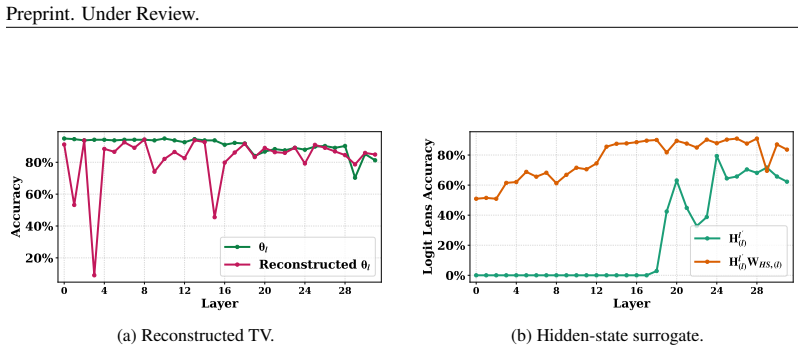
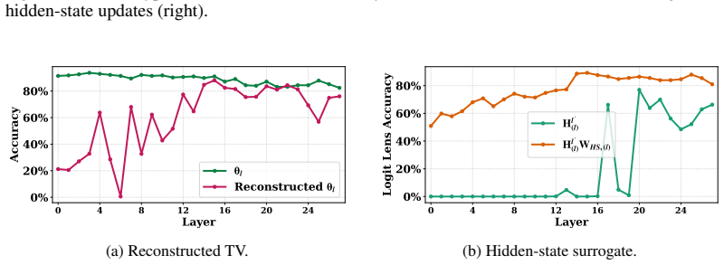
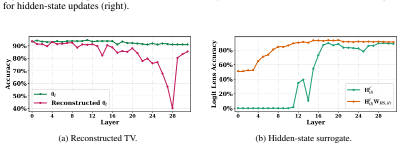
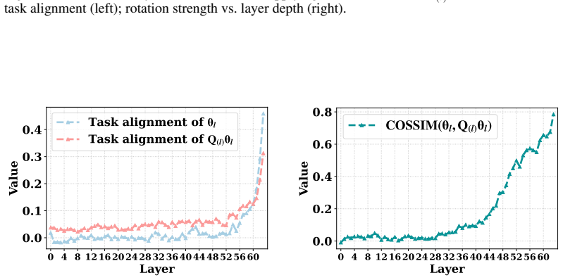
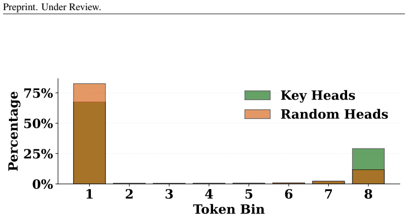
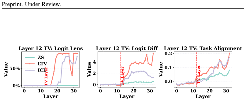
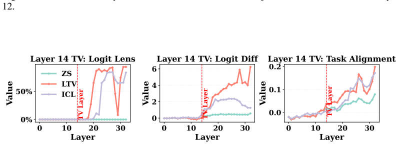
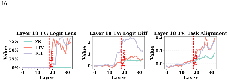
Directly trained Learned Task Vectors surpass extracted task vectors in accuracy and can be inserted at arbitrary layers, positions, and even together with standard in-context prompts. At the circuit level they steer predictions through attention-head OV circuits, with a small subset of key heads carrying most of the effect. Despite the nonlinearities inside transformers, the vectors propagate largely linearly: early vectors are rotated into task-relevant subspaces that raise the logits of relevant labels, while later vectors are scaled up in magnitude.
What carries the argument
Learned Task Vectors trained end-to-end to steer predictions, operating through attention-head OV circuits and propagating via early rotation toward task subspaces followed by later magnitude scaling.
If this is right
- Learned task vectors remain effective when inserted at any layer or token position.
- They continue to work when combined with ordinary in-context learning demonstrations.
- Prediction steering occurs primarily through the OV circuits of a small number of decisive attention heads.
- Early vectors improve relevant label logits by rotating into task subspaces; later vectors do so mainly by growing in magnitude.
Where Pith is reading between the lines
- The ability to train vectors separately could let practitioners optimize task representations without retraining the full model.
- The reported linear propagation may simplify future interventions that aim to edit or interpret task behavior inside transformers.
- If the pattern generalizes, similar training could be applied to control other emergent capabilities such as reasoning or tool use.
Load-bearing premise
The accuracy gains and the linear propagation pattern observed for trained vectors are not limited to the particular training procedure, model sizes, or tasks used in the experiments.
What would settle it
Retraining learned task vectors on a new collection of tasks or a different model family and finding that extracted vectors match or exceed them in accuracy, or measuring that interventions on nonlinear components substantially change the reported rotation-and-scaling pattern.
Figures


read the original abstract
Large Language Models (LLMs) can perform new tasks from in-context demonstrations, a phenomenon known as in-context learning (ICL). Recent work suggests that these demonstrations are compressed into task vectors (TVs), compact task representations that LLMs exploit for predictions. However, prior studies typically extract TVs from model outputs or hidden states using cumbersome and opaque methods, and they rarely elucidate the mechanisms by which TVs influence computation. In this work, we address both limitations. First, we propose directly training Learned Task Vectors (LTVs), which surpass extracted TVs in accuracy and exhibit superior flexibility-acting effectively at arbitrary layers, positions, and even with ICL prompts. Second, through systematic analysis, we investigate the mechanistic role of TVs, showing that at the low level they steer predictions primarily through attention-head OV circuits, with a small subset of "key heads" most decisive. At a higher level, we find that despite Transformer nonlinearities, TV propagation is largely linear: early TVs are rotated toward task-relevant subspaces to improve logits of relevant labels, while later TVs are predominantly scaled in magnitude. Taken together, LTVs not only provide a practical approach for obtaining effective TVs but also offer a principled lens into the mechanistic foundations of ICL.
Editorial analysis
A structured set of objections, weighed in public.
Referee Report
Summary. The manuscript proposes directly training Learned Task Vectors (LTVs) rather than extracting task vectors (TVs) from LLM hidden states or outputs for in-context learning. It claims LTVs achieve higher accuracy and greater flexibility (effective at arbitrary layers/positions and compatible with ICL prompts). Mechanistically, TVs steer predictions primarily via attention-head OV circuits (with a small subset of key heads decisive), and despite Transformer nonlinearities, propagation is largely linear: early TVs are rotated toward task-relevant subspaces to boost relevant label logits, while later TVs are mainly scaled in magnitude.
Significance. If the empirical and mechanistic claims hold under broader testing, the work supplies both a practical method for obtaining high-quality task representations and interpretable insights into ICL mechanisms. The direct-training approach and the OV-circuit plus linear-propagation findings could inform future control and analysis of transformer behavior.
major comments (4)
- [§4] §4 (Experiments): The central claim that trained LTVs surpass extracted TVs in accuracy and flexibility lacks explicit quantitative results, baseline comparisons, statistical significance tests, and controls for training-procedure artifacts in the reported overview; without these the degree of support for superiority cannot be assessed.
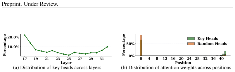
- [§5.2] §5.2 (Mechanistic analysis): The assertion that steering occurs primarily through attention-head OV circuits with a decisive subset of key heads requires ablation results quantifying performance drop when those heads are masked or removed; otherwise the circuit-level claim remains qualitative.
- [§6.1] §6.1 (Propagation analysis): The higher-level claim that TV propagation is 'largely linear' (early rotation to task subspaces, later magnitude scaling) despite nonlinearities needs explicit quantitative metrics such as cosine similarity to linear approximations or residual nonlinear error; absent these, the summary risks overstatement.
- [§4.3] §4.3 and §7 (Generalization): The observed performance and mechanistic advantages may be tied to the specific training objective, model family, or narrow task distribution; additional experiments across architectures and broader task sets are required to rule out artifacts and support the broader conclusions.
minor comments (2)
- [§2] Notation for extracted TVs versus LTVs should be introduced with a clear table or diagram in §2 to prevent reader confusion.
- [Figures] Figures showing key-head attention patterns and layer-wise propagation should include axis labels, error bars, and layer indices for immediate readability.
Simulated Author's Rebuttal
We thank the referee for the detailed and constructive report. We address each major comment below and describe the revisions we will incorporate to strengthen the empirical and mechanistic claims.
read point-by-point responses
-
Referee: [§4] §4 (Experiments): The central claim that trained LTVs surpass extracted TVs in accuracy and flexibility lacks explicit quantitative results, baseline comparisons, statistical significance tests, and controls for training-procedure artifacts in the reported overview; without these the degree of support for superiority cannot be assessed.
Authors: We agree that the main-text overview would benefit from greater explicitness. The manuscript already reports quantitative accuracy comparisons, baseline methods, and some statistical tests in the experimental section and appendices, but we will expand §4 to prominently feature key numerical results, direct baseline contrasts, significance testing, and controls for training-procedure artifacts so that the superiority claims can be evaluated directly from the main text. revision: yes
-
Referee: [§5.2] §5.2 (Mechanistic analysis): The assertion that steering occurs primarily through attention-head OV circuits with a decisive subset of key heads requires ablation results quantifying performance drop when those heads are masked or removed; otherwise the circuit-level claim remains qualitative.
Authors: We accept that the current identification of key heads via importance metrics would be strengthened by direct ablation. In the revised manuscript we will add ablation experiments that mask or remove the identified key heads and report the resulting performance drops, thereby providing quantitative support for their decisive role within the OV circuits. revision: yes
-
Referee: [§6.1] §6.1 (Propagation analysis): The higher-level claim that TV propagation is 'largely linear' (early rotation to task subspaces, later magnitude scaling) despite nonlinearities needs explicit quantitative metrics such as cosine similarity to linear approximations or residual nonlinear error; absent these, the summary risks overstatement.
Authors: We agree that additional quantitative grounding is warranted. We will augment §6.1 with explicit metrics, including cosine similarity between observed propagation trajectories and their linear approximations as well as measures of residual nonlinear error, to substantiate the characterization of propagation as largely linear. revision: yes
-
Referee: [§4.3] §4.3 and §7 (Generalization): The observed performance and mechanistic advantages may be tied to the specific training objective, model family, or narrow task distribution; additional experiments across architectures and broader task sets are required to rule out artifacts and support the broader conclusions.
Authors: We acknowledge the scope limitation. Our experiments prioritized depth of mechanistic analysis on standard models and tasks. In the revision we will add experiments on at least one additional architecture and an expanded task distribution to provide evidence that the reported advantages are not artifacts of the original experimental setting. revision: yes
Circularity Check
No significant circularity; empirical claims rest on training and analysis without definitional reduction
full rationale
The paper's core contribution is the proposal to directly train Learned Task Vectors (LTVs) rather than extract them, followed by empirical comparisons of accuracy and flexibility plus mechanistic dissection via attention OV circuits and observed linear propagation patterns. No equations, self-citations, or uniqueness theorems are invoked in the provided text that would make any performance gain or linearity claim equivalent to its inputs by construction. The derivation chain consists of experimental procedures and internal model analysis that remain independent of the target results; the claims are falsifiable via replication on different models or tasks and do not reduce to fitted parameters renamed as predictions or ansatzes smuggled through prior work.
Axiom & Free-Parameter Ledger
Lean theorems connected to this paper
-
IndisputableMonolith/Cost/FunctionalEquation.leanwashburn_uniqueness_aczel unclear?
unclearRelation between the paper passage and the cited Recognition theorem.
despite Transformer nonlinearities, TV propagation is largely linear: early TVs are rotated toward task-relevant subspaces ... later TVs are predominantly scaled in magnitude
-
IndisputableMonolith/Foundation/AbsoluteFloorClosure.leanabsolute_floor_iff_bare_distinguishability unclear?
unclearRelation between the paper passage and the cited Recognition theorem.
steer predictions primarily through attention-head OV circuits
What do these tags mean?
- matches
- The paper's claim is directly supported by a theorem in the formal canon.
- supports
- The theorem supports part of the paper's argument, but the paper may add assumptions or extra steps.
- extends
- The paper goes beyond the formal theorem; the theorem is a base layer rather than the whole result.
- uses
- The paper appears to rely on the theorem as machinery.
- contradicts
- The paper's claim conflicts with a theorem or certificate in the canon.
- unclear
- Pith found a possible connection, but the passage is too broad, indirect, or ambiguous to say the theorem truly supports the claim.
Reference graph
Works this paper leans on
-
[1]
Yi: Open foundation models by 01.ai, 2024
AI, Alex Young, Bei Chen, Chao Li, Chengen Huang, Ge Zhang, Guanwei Zhang, Heng Li, Jiangcheng Zhu, Jianqun Chen, Jing Chang, Kaidong Yu, Peng Liu, Qiang Liu, Shawn Yue, Senbin Yang, Shiming Yang, Tao Yu, Wen Xie, Wenhao Huang, Xiaohui Hu, Xiaoyi Ren, Xinyao Niu, Pengcheng Nie, Yuchi Xu, Yudong Liu, Yue Wang, Yuxuan Cai, Zhenyu Gu, Zhiyuan Liu, and Zongho...
-
[2]
Dongfang Li, Zhenyu Liu, Xinshuo Hu, Zetian Sun, Baotian Hu, and Min Zhang
URLhttps://arxiv.org/abs/2401.01967. Dongfang Li, Zhenyu Liu, Xinshuo Hu, Zetian Sun, Baotian Hu, and Min Zhang. In-context learning state vector with inner and momentum optimization, 2024a. URLhttps://arxiv.org/abs/ 2404.11225. Kenneth Li, Oam Patel, Fernanda Viégas, Hanspeter Pfister, and Martin Wattenberg. Inference- time intervention: Eliciting truthf...
-
[3]
Would you like a donut now, or two donuts in an hour?
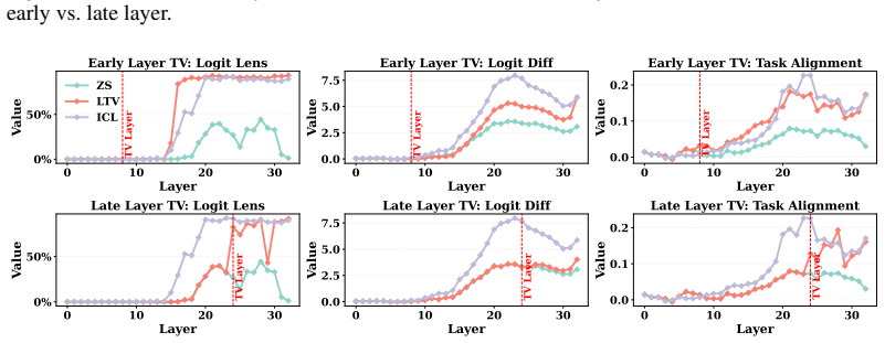
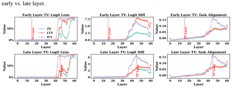
Interestingly, this is also the depth at which the Logit Lens Accuracy and Task Alignment values of the ICL hidden states begin to rise significantly above the zero-shot hidden state baselines. This is consistent with previous findings (Yang et al., 2025a), which report that ICL features a distinct transition pattern where hidden states increasingly align...
work page 2024
-
[6]
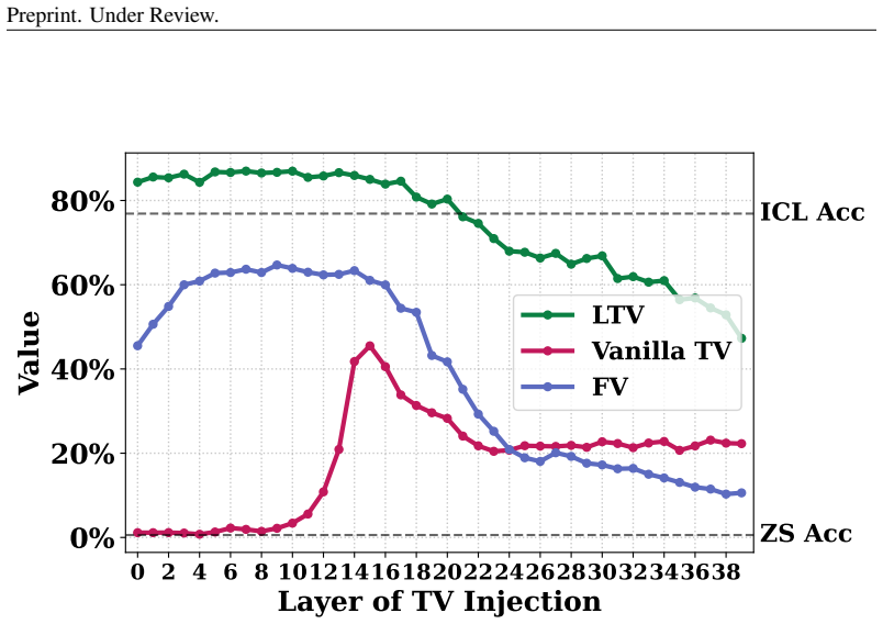
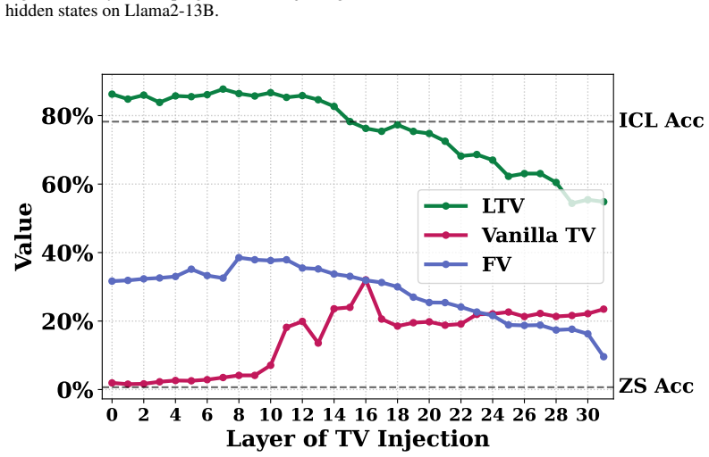
More layers & Pos. P={−5, . . .},L={0,2, . . .} 5) ICL prompts Vanilla TV 38.26% 1.96% 14.16% 18.85% 13.30% 52.82% FV 51.81% 1.40% 28.60% 47.14% 20.44% 73.23% LTV 82.54%↑30.73% 79.34%↑77.38% 84.60%↑56.00% 82.24%↑35.10% 51.60%↑31.16% 85.16%↑11.93% 22 Preprint. Under Review. 0 2 4 6 8 101214161820222426283032343638 Layer of TV Injection 0% 20% 40% 60% 80%Va...
-
[9]
More layers & Pos. P={−5, . . .},L={0,2, . . .} 5) ICL prompts Vanilla TV 27.67% 1.84% 16.42% 20.46% 16.07% 43.84% FV 41.59% 1.22% 42.25% 36.97% 24.74% 77.51% LTV 80.33%↑38.74% 71.53%↑69.69% 87.69%↑45.44% 82.25%↑45.28% 51.46%↑26.72% 84.99%↑7.48% 23 Preprint. Under Review. 0 2 4 6 8 10 12 14 16 18 20 22 24 26 Layer of TV Injection 0% 20% 40% 60% 80%Value Z...
-
[12]
More layers & Pos. P={−5, . . .},L={0,2, . . .} 5) ICL prompts Vanilla TV 31.69% 2.02% 1.05% 26.68% 0.33% 75.83% FV 33.28% 2.93% 18.38% 16.95% 17.72% 53.93% LTV 76.26%↑42.98% 76.22%↑73.29% 77.93%↑59.55% 83.48%↑56.80% 44.82%↑27.10% 84.51%↑8.68% Table 6: Comparison of LTV vs. FV and Vanilla TV across five scenarios on Llama3-8B. 24 Preprint. Under Review. I...
-
[15]
More layers & Pos. P={−5, . . .},L={0,2, . . .} 5) ICL prompts Vanilla TV 42.61% 3.07% 18.73% 37.05% 11.33% 65.38% FV 19.54% 3.53% 15.07% 4.69% 13.26% 62.12% LTV 78.65%↑36.04% 74.10%↑70.57% 78.18%↑59.45% 80.43%↑43.38% 46.38%↑33.12% 82.80%↑17.42% Table 7: Comparison of LTV vs. FV and Vanilla TV across five scenarios on Llama3.2-3B. Method Baseline P={−1},L={40}
-
[18]
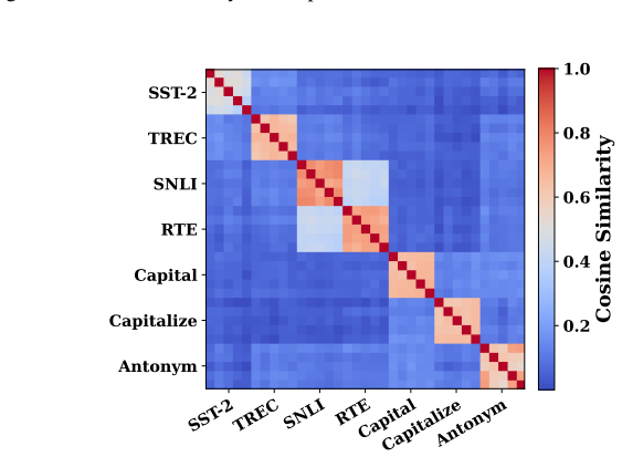
More layers & Pos. P={−5, . . .},L={0,2, . . .} 5) ICL prompts LTV 78.18% 75.34% 76.13% 75.59% 48.75% 88.40% Table 8: Performance of LTV across settings on Llama3-70B. 27 Preprint. Under Review. SST-2TRECSNLI RTE CapitalCapitalizeAntonym SST-2 TREC SNLI RTE Capital Capitalize Antonym 0.0 0.2 0.4 0.6 0.8 1.0 Cosine Similarity Figure 26: Cosine-similarity h...
-
[21]
More layers & Pos. P={−5, . . .},L={0,2, . . .} 5) ICL prompts LTV 75.59% 36.04% 75.20% 87.24% 53.30% 87.08% Table 9: Performance of LTV across settings on Qwen2.5-32B. Method Baseline P={−1},L={30}
-
[22]
More Pos. P={−5, . . . ,−1}
-
[23]
More layers L={0,4,8, . . .}
-
[24]
More layers & Pos. P={−5, . . .},L={0,2, . . .} 5) ICL prompts LTV 81.37% 73.53% 84.39% 82.47% 51.29% 89.69% Table 10: Performance of LTV across settings on Yi-34B. 28 Preprint. Under Review. SST-2TRECSNLI RTE CapitalCapitalizeAntonym SST-2 TREC SNLI RTE Capital Capitalize Antonym 0.2 0.4 0.6 0.8 1.0 Cosine Similarity Figure 28: Cosine-similarity heatmap ...
discussion (0)
Sign in with ORCID, Apple, or X to comment. Anyone can read and Pith papers without signing in.