STCast: Adaptive Boundary Alignment for Global and Regional Weather Forecasting
Pith reviewed 2026-05-18 15:07 UTC · model grok-4.3
The pith
STCast adapts regional boundaries from global weather fields using attention to improve forecast accuracy.
A machine-rendered reading of the paper's core claim, the machinery that carries it, and where it could break.
Core claim
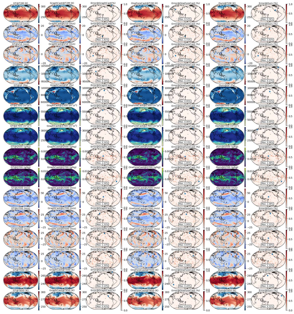
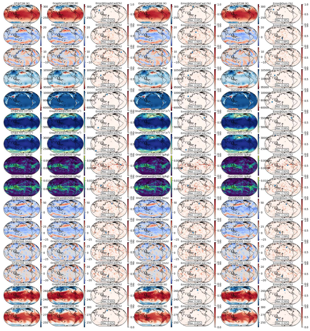
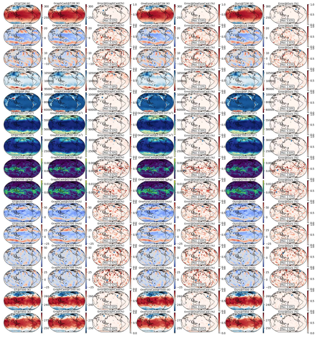
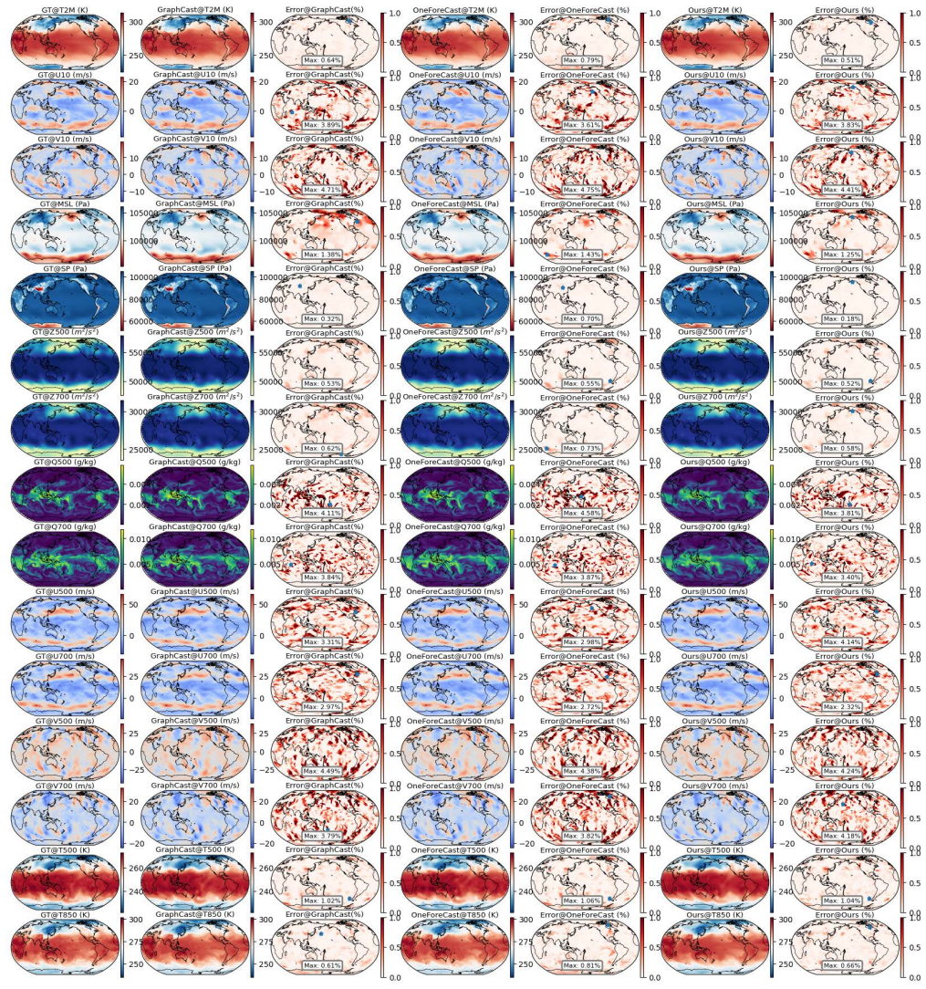
STCast employs a Spatial-Aligned Attention mechanism to initialize and then iteratively refine regional boundaries by aligning global and regional spatial distributions according to learned attention patterns. It pairs this with a Temporal Mixture-of-Experts module that routes atmospheric variables from distinct months through a discrete Gaussian distribution to specialized experts. When evaluated on global forecasting, regional forecasting, extreme event prediction, and ensemble forecasting, the resulting model shows consistent gains over prior state-of-the-art approaches across all four tasks.
What carries the argument
Spatial-Aligned Attention (SAA) mechanism that aligns global and regional spatial distributions to initialize and adaptively refine boundaries based on attention-derived patterns, paired with Temporal Mixture-of-Experts (TMoE) that routes monthly data to specialized experts via a discrete Gaussian distribution.
If this is right
- Regional forecasts can be generated without manually choosing fixed crop boundaries or solving separate physics boundary equations.
- The same trained model can handle both global-scale and regional-scale outputs by learning to adjust the interface between them.
- Monthly atmospheric patterns are captured more effectively when routed to distinct expert sub-networks instead of a single shared set of weights.
- Extreme event and ensemble prediction tasks benefit from the same adaptive boundary and temporal routing components without task-specific redesign.
Where Pith is reading between the lines
- The approach could be tested on climate projection ensembles where boundary conditions vary more strongly across decades.
- If the learned alignments prove stable, they might supply physically interpretable diagnostics for where global models lose skill at regional scales.
- Extending the routing logic beyond months to other slow-varying drivers such as ENSO phases could further reduce the need for separate models per regime.
Load-bearing premise
The attention-derived alignment patterns reflect physically meaningful and generalizable boundary adjustments rather than dataset-specific correlations.
What would settle it
Performance gains would disappear or reverse on a held-out test set drawn from different years, different geographic domains, or different climate regimes while keeping the same training distribution.
Figures


read the original abstract
To gain finer regional forecasts, many works have explored the regional integration from the global atmosphere, e.g., by solving boundary equations in physics-based methods or cropping regions from global forecasts in data-driven methods. However, the effectiveness of these methods is often constrained by static and imprecise regional boundaries, resulting in poor generalization ability. To address this issue, we propose Spatial-Temporal Weather Forecasting (STCast), a novel AI-driven framework for adaptive regional boundary optimization and dynamic monthly forecast allocation. Specifically, our approach employs a Spatial-Aligned Attention (SAA) mechanism, which aligns global and regional spatial distributions to initialize boundaries and adaptively refines them based on attention-derived alignment patterns. Furthermore, we design a Temporal Mixture-of-Experts (TMoE) module, where atmospheric variables from distinct months are dynamically routed to specialized experts using a discrete Gaussian distribution, enhancing the model's ability to capture temporal patterns. Beyond global and regional forecasting, we evaluate our STCast on extreme event prediction and ensemble forecasting. Experimental results demonstrate consistent superiority over state-of-the-art methods across all four tasks. Code: https://github.com/chenhao-zju/STCast
Editorial analysis
A structured set of objections, weighed in public.
Referee Report
Summary. The paper proposes STCast, an AI-driven framework for weather forecasting that introduces a Spatial-Aligned Attention (SAA) module to adaptively align global and regional spatial distributions and refine boundaries based on attention patterns, along with a Temporal Mixture-of-Experts (TMoE) module that routes atmospheric variables from distinct months to specialized experts via a discrete Gaussian distribution. The model is evaluated on global and regional forecasting, extreme event prediction, and ensemble forecasting, with the central claim being consistent superiority over state-of-the-art methods across all four tasks.
Significance. If the adaptive boundary alignment proves robust and generalizable beyond the training distribution, the work could meaningfully advance data-driven regional weather forecasting by overcoming limitations of static boundaries in both physics-based and ML approaches, with potential benefits for extreme event and ensemble predictions.
major comments (2)
- [§3.1] §3.1 (SAA module description): The central generalization claim across the four tasks rests on the assumption that attention-derived alignment patterns produce physically meaningful and robust boundary adjustments. No analysis is provided (e.g., attention map visualizations compared to known meteorological fronts, or explicit distribution-shift experiments) to distinguish these patterns from dataset-specific statistical correlations, which directly bears on whether the reported gains will hold on independent test sets.
- [§4] §4 (Experimental results): While consistent outperformance is asserted, the section lacks reported details on dataset sizes, exact error metrics with confidence intervals, statistical significance tests, and full ablation controls for the SAA and TMoE components; without these, it is difficult to rule out that gains arise from hyperparameter tuning differences rather than the proposed modules.
minor comments (2)
- [§3.2] The notation for the discrete Gaussian distribution in the TMoE routing could be clarified with an explicit equation or pseudocode to aid reproducibility.
- [Figures] Figure captions for attention visualizations (if present) should explicitly state the color scale and what the highlighted regions represent in physical terms.
Simulated Author's Rebuttal
We thank the referee for the constructive and detailed feedback. We address each major comment below and outline the revisions planned for the manuscript.
read point-by-point responses
-
Referee: [§3.1] §3.1 (SAA module description): The central generalization claim across the four tasks rests on the assumption that attention-derived alignment patterns produce physically meaningful and robust boundary adjustments. No analysis is provided (e.g., attention map visualizations compared to known meteorological fronts, or explicit distribution-shift experiments) to distinguish these patterns from dataset-specific statistical correlations, which directly bears on whether the reported gains will hold on independent test sets.
Authors: We agree that additional evidence is required to substantiate that the attention patterns yield physically meaningful boundary adjustments rather than dataset-specific correlations. In the revised manuscript we will include visualizations of SAA attention maps overlaid on standard meteorological fields and compare them against documented fronts and boundaries. We will also add distribution-shift experiments using held-out years and geographically distinct regions to evaluate robustness outside the original training distribution. revision: yes
-
Referee: [§4] §4 (Experimental results): While consistent outperformance is asserted, the section lacks reported details on dataset sizes, exact error metrics with confidence intervals, statistical significance tests, and full ablation controls for the SAA and TMoE components; without these, it is difficult to rule out that gains arise from hyperparameter tuning differences rather than the proposed modules.
Authors: We acknowledge that the current experimental section would benefit from greater rigor. In the revision we will report exact training and test dataset sizes, present all primary metrics together with confidence intervals obtained from multiple random seeds, include statistical significance tests (paired t-tests) against baselines, and expand the ablation studies to fully isolate the contributions of SAA and TMoE while controlling for hyperparameter budgets. revision: yes
Circularity Check
No circularity: empirical ML framework with independent experimental validation
full rationale
The paper introduces STCast as a neural architecture combining Spatial-Aligned Attention for adaptive boundaries and Temporal Mixture-of-Experts for monthly routing. All load-bearing claims are empirical performance gains on global/regional forecasting, extremes, and ensembles, measured against external baselines on held-out data. No derivation, uniqueness theorem, or first-principles result is presented that reduces by construction to fitted parameters, self-citations, or renamed inputs. The SAA and TMoE modules are standard attention and MoE designs applied to weather tensors; their effectiveness is tested rather than assumed via internal redefinition. This is a self-contained empirical contribution with no detectable circular steps.
Axiom & Free-Parameter Ledger
free parameters (2)
- number of experts in TMoE
- attention temperature or scaling factor in SAA
axioms (2)
- domain assumption Atmospheric fields at global and regional scales share sufficient spatial structure that attention can recover meaningful boundary adjustments.
- domain assumption Monthly atmospheric variables are sufficiently distinct that routing them to separate experts improves temporal modeling.
invented entities (2)
-
Spatial-Aligned Attention (SAA) module
no independent evidence
-
Temporal Mixture-of-Experts (TMoE) module
no independent evidence
Lean theorems connected to this paper
-
IndisputableMonolith/Cost/FunctionalEquation.leanwashburn_uniqueness_aczel unclear?
unclearRelation between the paper passage and the cited Recognition theorem.
Spatial-Aligned Attention (SAA) ... Manhattan distance ... exponential distance-decay function ... Hadamard product between the initial global-regional distribution and the attention map
What do these tags mean?
- matches
- The paper's claim is directly supported by a theorem in the formal canon.
- supports
- The theorem supports part of the paper's argument, but the paper may add assumptions or extra steps.
- extends
- The paper goes beyond the formal theorem; the theorem is a base layer rather than the whole result.
- uses
- The paper appears to rely on the theorem as machinery.
- contradicts
- The paper's claim conflicts with a theorem or certificate in the canon.
- unclear
- Pith found a possible connection, but the passage is too broad, indirect, or ambiguous to say the theorem truly supports the claim.
Forward citations
Cited by 2 Pith papers
-
SwAIther-Precip: Lead-Time-Aware Bias Correction Enables Kilometer-Scale Downscaling of Global AI Precipitation Forecasts over Switzerland
SwAIther-Precip uses lead-time-conditioned U-Net bias correction followed by diffusion-based super-resolution to downscale AIFS forecasts, achieving 48% CRPS reduction and ~4 km effective resolution up to 5 days lead time.
-
Generative 3D Gaussian Splatting for Arbitrary-ResolutionAtmospheric Downscaling and Forecasting
A generative 3D Gaussian splatting model with scale-aware attention enables unified arbitrary-resolution forecasting and downscaling of 87 atmospheric variables.
Reference graph
Works this paper leans on
-
[1]
, " * write output.state after.block = add.period write newline
ENTRY address archivePrefix author booktitle chapter edition editor eid eprint howpublished institution isbn journal key month note number organization pages publisher school series title type volume year label extra.label sort.label short.list INTEGERS output.state before.all mid.sentence after.sentence after.block FUNCTION init.state.consts #0 'before.a...
-
[2]
" write newline "" before.all 'output.state := FUNCTION n.dashify 't := "" t empty not t #1 #1 substring "-" = t #1 #2 substring "--" = not "--" * t #2 global.max substring 't := t #1 #1 substring "-" = "-" * t #2 global.max substring 't := while if t #1 #1 substring * t #2 global.max substring 't := if while FUNCTION word.in bbl.in capitalize " " * FUNCT...
-
[3]
Adamov, S.; Oskarsson, J.; Denby, L.; Landelius, T.; Hintz, K.; Christiansen, S.; Schicker, I.; Osuna, C.; Lindsten, F.; Fuhrer, O.; et al. 2025. Building Machine Learning Limited Area Models: Kilometer-Scale Weather Forecasting in Realistic Settings. arXiv preprint arXiv:2504.09340
-
[4]
Bauer, P.; Thorpe, A.; and Brunet, G. 2015. The quiet revolution of numerical weather prediction. Nature, 525(7567): 47--55
work page 2015
-
[5]
Bi, K.; Xie, L.; Zhang, H.; Chen, X.; Gu, X.; and Tian, Q. 2023. Accurate medium-range global weather forecasting with 3D neural networks. Nature, 619(7970): 533--538
work page 2023
-
[6]
Bodnar, C.; Bruinsma, W. P.; Lucic, A.; Stanley, M.; Brandstetter, J.; Garvan, P.; Riechert, M.; Weyn, J.; Dong, H.; Vaughan, A.; et al. 2025. Aurora: A foundation model of the atmosphere. Nature, 641: 1180--1187
work page 2025
-
[7]
Bonev, B.; Kurth, T.; Hundt, C.; Pathak, J.; Baust, M.; Kashinath, K.; and Anandkumar, A. 2023. Spherical Fourier neural operators: learning stable dynamics on the sphere. In Proceedings of the 40th International Conference on Machine Learning
work page 2023
-
[8]
Chen, H.; Tao, H.; Song, G.; Zhang, J.; Yu, Y.; Dong, Y.; and Bai, L. 2025. VA-MoE: Variables-Adaptive Mixture of Experts for Incremental Weather Forecasting. In Proceedings of the IEEE/CVF International Conference on Computer Vision (ICCV)
work page 2025
- [9]
-
[10]
Chen, L.; Zhong, X.; Zhang, F.; Cheng, Y.; Xu, Y.; Qi, Y.; and Li, H. 2023 b . FuXi: A cascade machine learning forecasting system for 15-day global weather forecast. npj Climate and Atmospheric Science, 6(1): 190
work page 2023
- [11]
-
[12]
Dao, T.; Fu, D.; Ermon, S.; Rudra, A.; and R \'e , C. 2022. Flashattention: Fast and memory-efficient exact attention with io-awareness. In Advances in Neural Information Processing Systems, volume 35, 16344--16359
work page 2022
-
[13]
Gan, L.; Man, X.; Zhang, C.; and Shao, J. 2025. EWMoE: An effective model for global weather forecasting with mixture-of-experts. In Proceedings of the AAAI Conference on Artificial Intelligence, volume 39, 210--218
work page 2025
-
[14]
Gao, Y.; Wu, H.; Shu, R.; Dong, H.; Xu, F.; Chen, R.; Yan, Y.; Wen, Q.; Hu, X.; Wang, K.; et al. 2025. OneForecast: A Universal Framework for Global and Regional Weather Forecasting. In Proceedings of the 42th International Conference on Machine Learning
work page 2025
-
[15]
Gao, Z.; Tan, C.; Wu, L.; and Li, S. Z. 2022. Simvp: Simpler yet better video prediction. In Proceedings of the IEEE/CVF conference on computer vision and pattern recognition, 3170--3180
work page 2022
-
[16]
Gong, Y.; He, T.; Chen, M.; Wang, B.; Nie, L.; and Yin, Y. 2024. Spatio-temporal enhanced contrastive and contextual learning for weather forecasting. IEEE Transactions on Knowledge and Data Engineering, 36(8): 4260--4274
work page 2024
- [17]
-
[18]
He, J.; Ji, J.; and Lei, M. 2024. Spatio-temporal transformer network with physical knowledge distillation for weather forecasting. In Proceedings of the 33rd ACM International Conference on Information and Knowledge Management, 819--828
work page 2024
-
[19]
Hersbach, H.; Bell, B.; Berrisford, P.; Hirahara, S.; Hor \'a nyi, A.; Mu \ n oz-Sabater, J.; Nicolas, J.; Peubey, C.; Radu, R.; Schepers, D.; et al. 2020. The ERA5 global reanalysis. Quarterly Journal of the Royal Meteorological Society, 146(730): 1999--2049
work page 2020
-
[20]
Hidayatullah, A. F.; Aditya, S. K.; Gardini, S. T.; et al. 2019. Topic modeling of weather and climate condition on twitter using latent dirichlet allocation (LDA). In IOP Conference Series: Materials Science and Engineering, volume 482, 012033
work page 2019
-
[21]
Ji, J.; He, J.; Lei, M.; Wang, M.; and Tang, W. 2024. Spatio-temporal transformer network for weather forecasting. IEEE Transactions on Big Data, 11(2): 372--387
work page 2024
-
[22]
Kalnay, E. 2002. Atmospheric modeling, data assimilation and predictability. Cambridge: Cambridge University Press
work page 2002
- [23]
-
[24]
Kurth, T.; Subramanian, S.; Harrington, P.; Pathak, J.; Mardani, M.; Hall, D.; Miele, A.; Kashinath, K.; and Anandkumar, A. 2023. FourCastNet: Accelerating Global High-Resolution Weather Forecasting Using Adaptive Fourier Neural Operators. In Proceedings of the Platform for Advanced Scientific Computing Conference, PASC '23
work page 2023
-
[25]
Lam, R.; Sanchez-Gonzalez, A.; Willson, M.; Wirnsberger, P.; Fortunato, M.; Alet, F.; Ravuri, S.; Ewalds, T.; Eaton-Rosen, Z.; Hu, W.; et al. 2023. Learning skillful medium-range global weather forecasting. Science, 382(6677): 1416--1421
work page 2023
-
[26]
B.; Azizzadenesheli, K.; liu, B.; Bhattacharya, K.; Stuart, A.; and Anandkumar, A
Li, Z.; Kovachki, N. B.; Azizzadenesheli, K.; liu, B.; Bhattacharya, K.; Stuart, A.; and Anandkumar, A. 2021. Fourier Neural Operator for Parametric Partial Differential Equations. In International Conference on Learning Representations
work page 2021
-
[27]
Liu, Z.; Lin, Y.; Cao, Y.; Hu, H.; Wei, Y.; Zhang, Z.; Lin, S.; and Guo, B. 2021. Swin transformer: Hierarchical vision transformer using shifted windows. In Proceedings of the IEEE/CVF International Conference on Computer Vision (ICCV), 10012--10022
work page 2021
-
[28]
Lu, X.; Yu, H.; Ying, M.; Zhao, B.; Zhang, S.; Lin, L.; Bai, L.; and Wan, R. 2021. Western North Pacific tropical cyclone database created by the China Meteorological Administration. Advances in Atmospheric Sciences, 38(4): 690--699
work page 2021
-
[29]
Lundquist, K. A.; Chow, F. K.; and Lundquist, J. K. 2010. An immersed boundary method for the weather research and forecasting model. Monthly Weather Review, 138(3): 796--817
work page 2010
-
[30]
Lynch, P. 2008. The origins of computer weather prediction and climate modeling. Journal of computational physics, 227(7): 3431--3444
work page 2008
-
[31]
Ma, M.; Xie, P.; Teng, F.; Wang, B.; Ji, S.; Zhang, J.; and Li, T. 2023. HiSTGNN: Hierarchical spatio-temporal graph neural network for weather forecasting. Information Sciences, 648: 119580
work page 2023
-
[32]
Magnusson, L.; Majumdar, S.; Emerton, R.; Richardson, D.; Alonso-Balmaseda, M.; Baugh, C.; Bechtold, P.; Bidlot, J.; Bonanni, A.; Bonavita, M.; et al. 2021. Tropical cyclone activities at ECMWF. ECMWF Technical Memoranda
work page 2021
-
[33]
Manabe, S.; and Bryan, K. 1969. Climate calculations with a combined ocean-atmosphere model. Journal of Atmospheric Sciences, 26(4): 786--789
work page 1969
-
[34]
Mani, A. 2012. Analysis and optimization of numerical sponge layers as a nonreflective boundary treatment. Journal of Computational Physics, 231(2): 704--716
work page 2012
-
[35]
Molteni, F.; Buizza, R.; Palmer, T. N.; and Petroliagis, T. 1996. The ECMWF ensemble prediction system: Methodology and validation. Quarterly journal of the royal meteorological society, 122(529): 73--119
work page 1996
-
[36]
Nguyen, T.; Brandstetter, J.; Kapoor, A.; Gupta, J. K.; and Grover, A. 2023. ClimaX: A foundation model for weather and climate. In International Conference on Machine Learning
work page 2023
-
[37]
Nguyen, T.; Shah, R.; Bansal, H.; Arcomano, T.; Maulik, R.; Kotamarthi, R.; Foster, I.; Madireddy, S.; and Grover, A. 2025. Scaling transformer neural networks for skillful and reliable medium-range weather forecasting. In Advances in Neural Information Processing Systems, volume 37, 68740--68771
work page 2025
-
[38]
Nipen, T. N.; Haugen, H. H.; Ingstad, M. S.; Nordhagen, E. M.; Salihi, A. F. S.; Tedesco, P.; Seierstad, I. A.; Kristiansen, J.; Lang, S.; Alexe, M.; et al. 2024. Regional data-driven weather modeling with a global stretched-grid. arXiv preprint arXiv:2409.02891
-
[39]
R.; El-Kadi, A.; Masters, D.; Ewalds, T.; Stott, J.; Mohamed, S.; Battaglia, P.; et al
Price, I.; Sanchez-Gonzalez, A.; Alet, F.; Andersson, T. R.; El-Kadi, A.; Masters, D.; Ewalds, T.; Stott, J.; Mohamed, S.; Battaglia, P.; et al. 2025. Probabilistic weather forecasting with machine learning. Nature, 637(8044): 84--90
work page 2025
-
[40]
Rasp, S.; Hoyer, S.; Merose, A.; Langmore, I.; Battaglia, P.; Russell, T.; Sanchez-Gonzalez, A.; Yang, V.; Carver, R.; Agrawal, S.; et al. 2024. WeatherBench 2: A benchmark for the next generation of data-driven global weather models. Journal of Advances in Modeling Earth Systems, 16(6): e2023MS004019
work page 2024
-
[41]
Ritchie, H.; Temperton, C.; Simmons, A.; Hortal, M.; Davies, T.; Dent, D.; and Hamrud, M. 1995. Implementation of the semi-Lagrangian method in a high-resolution version of the ECMWF forecast model. Monthly Weather Review, 123(2): 489--514
work page 1995
-
[42]
Sabathier, M.; Pannekoucke, O.; Maget, V.; and Dahmen, N. 2023. Boundary conditions for the parametric Kalman filter forecast. Journal of Advances in Modeling Earth Systems, 15(10): e2022MS003462
work page 2023
-
[43]
Shazeer, N.; Mirhoseini, A.; Maziarz, K.; Davis, A.; Le, Q.; Hinton, G.; and Dean, J. 2017. Outrageously large neural networks: The sparsely-gated mixture-of-experts layer. In International Conference on Learning Representations
work page 2017
-
[44]
Z.; Separovic, L.; and Yang, J
Subich, C.; Husain, S. Z.; Separovic, L.; and Yang, J. 2025. Fixing the double penalty in data-driven weather forecasting through a modified spherical harmonic loss function. In Proceedings of the 42th International Conference on Machine Learning
work page 2025
-
[45]
Veillette, M.; Samsi, S.; and Mattioli, C. 2020. Sevir: A storm event imagery dataset for deep learning applications in radar and satellite meteorology. In Advances in Neural Information Processing Systems, volume 33, 22009--22019
work page 2020
-
[46]
Verma, Y.; Heinonen, M.; and Garg, V. 2024. Clim ODE : Climate Forecasting With Physics-informed Neural ODE s. In International Conference on Learning Representations
work page 2024
-
[47]
Wang, B.; Lu, J.; Yan, Z.; Luo, H.; Li, T.; Zheng, Y.; and Zhang, G. 2019. Deep Uncertainty Quantification: A Machine Learning Approach for Weather Forecasting. In Proceedings of the 25th ACM SIGKDD International Conference on Knowledge Discovery & Data Mining, 2087–2095
work page 2019
-
[48]
Wang, X.; Chen, K.; Liu, L.; Han, T.; Li, B.; and Bai, L. 2025 a . Global tropical cyclone intensity forecasting with multi-modal multi-scale causal autoregressive model. In ICASSP 2025-2025 IEEE International Conference on Acoustics, Speech and Signal Processing (ICASSP), 1--5. IEEE
work page 2025
-
[49]
Wang, X.; Liu, L.; Chen, K.; Han, T.; Li, B.; and Bai, L. 2025 b . VQLTI: Long-Term Tropical Cyclone Intensity Forecasting with Physical Constraints. In Proceedings of the AAAI Conference on Artificial Intelligence, volume 39, 28476--28484
work page 2025
-
[50]
Wu, B.; Chen, W.; Wang, W.; Peng, B.; Sun, L.; and Chen, L. 2025. Weathergnn: Exploiting meteo-and spatial-dependencies for local numerical weather prediction bias-correction. In International Joint Conference on Artificial Intelligence
work page 2025
-
[51]
Wu, G.; Zhou, X.; Xu, X.; Huang, J.; Duan, A.; Yang, S.; Hu, W.; Ma, Y.; Liu, Y.; Bian, J.; et al. 2023. An integrated research plan for the Tibetan Plateau land--air coupled system and its impacts on the global climate. Bulletin of the American Meteorological Society, 104(1): E158--E177
work page 2023
-
[52]
Wu, H.; Weng, K.; Zhou, S.; Huang, X.; and Xiong, W. 2024 a . Neural manifold operators for learning the evolution of physical dynamics. In Proceedings of the 30th ACM SIGKDD Conference on Knowledge Discovery and Data Mining, 3356--3366
work page 2024
-
[53]
Wu, H.; Xu, F.; Chen, C.; Hua, X.-S.; Luo, X.; and Wang, H. 2024 b . Pastnet: Introducing physical inductive biases for spatio-temporal video prediction. In Proceedings of the 32nd ACM international conference on multimedia, 2917--2926
work page 2024
-
[54]
Xiong, W.; Ma, M.; Huang, X.; Zhang, Z.; Sun, P.; and Tian, Y. 2023. Koopmanlab: machine learning for solving complex physics equations. APL Machine Learning, 1(3)
work page 2023
-
[55]
Xu, W.; Ling, F.; Zhang, W.; Han, T.; Chen, H.; Ouyang, W.; and Bai, L. 2024. Generalizing Weather Forecast to Fine-grained Temporal Scales via Physics-AI Hybrid Modeling. In Advances in Neural Information Processing Systems
work page 2024
-
[56]
Ying, M.; Zhang, W.; Yu, H.; Lu, X.; Feng, J.; Fan, Y.; Zhu, Y.; and Chen, D. 2014. An overview of the China Meteorological Administration tropical cyclone database. Journal of Atmospheric and Oceanic Technology, 31(2): 287--301
work page 2014
-
[57]
Zhang, R.-H.; Tian, F.; and Wang, X. 2018. Ocean chlorophyll-induced heating feedbacks on ENSO in a coupled ocean physics--biology model forced by prescribed wind anomalies. Journal of Climate, 31(5): 1811--1832
work page 2018
discussion (0)
Sign in with ORCID, Apple, or X to comment. Anyone can read and Pith papers without signing in.