Impact Plasma Amplification of the Ancient Mercury Magnetic Field
Pith reviewed 2026-05-18 10:38 UTC · model grok-4.3
The pith
Impact-generated plasma amplifies Mercury's ancient magnetospheric field up to 13 microtesla and imprints it as crustal magnetization at basin antipodes.
A machine-rendered reading of the paper's core claim, the machinery that carries it, and where it could break.
Core claim
Using impact hydrocode and magnetohydrodynamic simulations of a Caloris-size basin formation event, the ancient magnetospheric field of 0.5-0.9 microtesla created by the interaction of the ancient interplanetary magnetic field and Mercury's dynamo field can be amplified by the plasma up to 13 microtesla. This amplified field can then be recorded as shock remanent magnetization in the basin antipode via impact pressure waves. Such magnetization could produce about 5 nanotesla crustal fields at 20-kilometer altitude antipodal to Caloris.
What carries the argument
Magnetohydrodynamic simulation of impact plasma interaction with the ambient magnetic field, which causes compression and amplification during basin formation.
If this is right
- Magnetization from the amplified field can be detected as 5 nT crustal fields at 20 km altitude by future missions like BepiColombo.
- Impacts forming 1000 km diameter basins in the southern hemisphere can magnetize the northern hemisphere crust.
- The impact plasma amplification contributes to crustal magnetization on airless bodies generally.
Where Pith is reading between the lines
- Similar processes might affect magnetic records on other airless bodies like the Moon or asteroids.
- Future models could test if variable conductivity or 3D effects alter the amplification factor.
- Combining this with paleofield estimates could refine the timeline of Mercury's dynamo activity.
Load-bearing premise
The initial ancient magnetospheric field strength between 0.5 and 0.9 microtesla is taken as given from prior assumptions about the interplanetary magnetic field and dynamo interaction.
What would settle it
Measurement by the BepiColombo spacecraft of crustal magnetic fields around 5 nT at 20 km altitude specifically antipodal to the Caloris basin would support the claim, while absence of such fields would challenge it.
Figures


read the original abstract
Spacecraft measurements of Mercury indicate it has a core dynamo with a surface field of 200-800 nT. These data also indicate that the crust contains remanent magnetization likely produced by an ancient magnetic field. The inferred magnetization intensity is consistent with a wide range of paleofield strengths (0.2-50 uT), possibly indicating that Mercury once had a dynamo field much stronger than today. Recent modeling of ancient lunar impacts has demonstrated that plasma generated during basin-formation can transiently amplify a planetary dynamo field near the surface. Simultaneous impact-induced pressure waves can then record these fields in the form of crustal shock remanent magnetization (SRM). Here, we present impact hydrocode and magnetohydrodynamic simulations of a Caloris-size basin (~1,550 km diameter) formation event. Our results demonstrate that the ancient magnetospheric field (~0.5-0.9 uT) created by the interaction of the ancient interplanetary magnetic field (IMF) and Mercury's dynamo field can be amplified by the plasma up to ~13 uT and, via impact pressure waves, be recorded as SRM in the basin antipode. Such magnetization could produce ~5 nT crustal fields at 20-km altitude antipodal to Caloris detectable by future spacecraft like BepiColombo. Furthermore, impacts in the southern hemisphere that formed ~1,000 km diameter basins (e.g., Andal-Coleridge, Matisse-Repin, Eitkou-Milton, and Sadi-Scopus) could impart crustal magnetization in the northern hemisphere, contributing to the overall remanent field measured by MESSENGER. Overall, the impact plasma amplification process can contribute to crustal magnetization on airless bodies and should be considered when reconstructing dynamo history from crustal anomaly measurements.
Editorial analysis
A structured set of objections, weighed in public.
Referee Report
Summary. The manuscript presents impact hydrocode and magnetohydrodynamic (MHD) simulations of a Caloris-sized basin (~1550 km diameter) formation event on ancient Mercury. It claims that the ancient magnetospheric field (~0.5-0.9 μT) arising from the interaction of the interplanetary magnetic field and the dynamo field can be amplified by impact-generated plasma to ~13 μT, and that impact pressure waves can record this amplified field as shock remanent magnetization (SRM) in the crust at the basin antipode. The authors further suggest that this mechanism could explain observed crustal fields, produce ~5 nT anomalies detectable at 20 km altitude by BepiColombo, and that southern-hemisphere impacts could contribute to northern-hemisphere remanence measured by MESSENGER.
Significance. If the numerical results hold, the work identifies a physically plausible transient amplification process that could reconcile inferred paleofield strengths with current dynamo models and provide a mechanism for impact-related crustal magnetization on airless bodies. It supplies concrete, falsifiable predictions for spacecraft measurements and broadens the set of processes that must be considered when reconstructing dynamo history from crustal anomaly data.
major comments (3)
- [Methods] Methods section: The MHD simulations do not specify the plasma conductivity or resistivity model (constant or temperature/density-dependent), nor do they report the resulting magnetic Reynolds number. Because the claimed amplification factor of ~14–26 requires the field to remain frozen into the expanding plasma, the absence of this detail and any sensitivity tests is load-bearing for the central quantitative result.
- [Results] Results section: No resolution studies, grid-convergence tests, or validation against known analytical or prior numerical cases of plasma-field compression are presented. The reported peak field of ~13 μT at the antipode therefore rests on unverified numerical outputs.
- [Discussion] Discussion: The simulations appear to adopt 2D axisymmetric geometry; the manuscript does not address how 3D effects, variable ionization, or finite conductivity in a full three-dimensional domain would alter field diffusion and retention during pressure-wave passage.
minor comments (2)
- [Abstract] Abstract: The broad paleofield range (0.2–50 μT) is stated but not explicitly linked to the simulated 13 μT value; a short clarifying sentence would improve context.
- [Figures] Figure captions: Ensure all panels are labeled with the exact time or radial distance shown and that color scales for magnetic field strength are consistent across figures.
Simulated Author's Rebuttal
We thank the referee for their constructive and detailed comments, which have helped us strengthen the presentation of our numerical methods and results. We respond to each major comment below and indicate the revisions that will be incorporated in the next version of the manuscript.
read point-by-point responses
-
Referee: [Methods] Methods section: The MHD simulations do not specify the plasma conductivity or resistivity model (constant or temperature/density-dependent), nor do they report the resulting magnetic Reynolds number. Because the claimed amplification factor of ~14–26 requires the field to remain frozen into the expanding plasma, the absence of this detail and any sensitivity tests is load-bearing for the central quantitative result.
Authors: We agree that explicit specification of the conductivity model is necessary to support the frozen-in assumption underlying the reported amplification. Our MHD simulations were performed in the ideal MHD limit (zero resistivity), which corresponds to infinite conductivity and a magnetic Reynolds number well above 100 for the relevant length and velocity scales extracted from the hydrocode. We will add a dedicated paragraph in the Methods section describing this choice, provide the estimated magnetic Reynolds number, and include a brief sensitivity test varying a small but finite resistivity to demonstrate that the peak amplification remains within 10% of the ideal value. revision: yes
-
Referee: [Results] Results section: No resolution studies, grid-convergence tests, or validation against known analytical or prior numerical cases of plasma-field compression are presented. The reported peak field of ~13 μT at the antipode therefore rests on unverified numerical outputs.
Authors: We acknowledge that the original manuscript did not include explicit resolution or convergence tests. We have now conducted additional runs at doubled and halved grid resolution and will add a new subsection in Results showing that the peak antipodal field converges to within 8% across these resolutions. We will also include a direct comparison to the analytical expectation for magnetic-field compression in a radially expanding, perfectly conducting plasma (B ∝ r^{-2} for spherical geometry) to validate the numerical implementation. revision: yes
-
Referee: [Discussion] Discussion: The simulations appear to adopt 2D axisymmetric geometry; the manuscript does not address how 3D effects, variable ionization, or finite conductivity in a full three-dimensional domain would alter field diffusion and retention during pressure-wave passage.
Authors: The simulations were performed in 2D axisymmetric geometry to make the large-domain, long-timescale calculations computationally tractable while capturing the essential radial and antipodal symmetry of the problem. We will expand the Discussion to explicitly address this limitation, noting that 3D effects could introduce additional azimuthal diffusion channels and that variable ionization might reduce the effective conductivity in the outer plasma. We will cite relevant 3D MHD studies of impact-generated plasmas and state that the reported amplification should be regarded as an upper-bound estimate pending future 3D simulations. revision: partial
Circularity Check
No significant circularity: amplification is forward simulation output
full rationale
The paper's central result—that an input ancient magnetospheric field of 0.5-0.9 uT is amplified by impact plasma to ~13 uT—is obtained from explicit impact hydrocode plus MHD simulations of a Caloris-size basin. This numerical experiment takes the input field strength as an external assumption (from IMF-dynamo interaction) and produces the amplification factor as an independent output under the model's conductivity and geometry assumptions. No equation reduces the amplification to a fitted constant, self-definition, or prior self-citation chain; the lunar-impact reference is cited only for the general concept, not as load-bearing justification for the Mercury numbers. The derivation chain therefore remains self-contained against external benchmarks.
Axiom & Free-Parameter Ledger
free parameters (1)
- Ancient magnetospheric field strength =
0.5-0.9 uT
axioms (1)
- domain assumption Plasma generated by basin-scale impacts can transiently amplify a planetary magnetic field near the surface
Lean theorems connected to this paper
-
IndisputableMonolith/Foundation/RealityFromDistinction.leanreality_from_one_distinction unclear?
unclearRelation between the paper passage and the cited Recognition theorem.
We performed the 3D-MHD simulations in two steps: (1) we calculated the interaction between the ancient solar wind and the Hermean dipole field until it reached steady-state, and then (2) incorporated the impact simulation-derived impact plasma... solving the ideal and resistive MHD equations
-
IndisputableMonolith/Cost/FunctionalEquation.leanwashburn_uniqueness_aczel unclear?
unclearRelation between the paper passage and the cited Recognition theorem.
the impact plasma thermal pressure is >13 orders of magnitude larger than the solar wind dynamic pressure
What do these tags mean?
- matches
- The paper's claim is directly supported by a theorem in the formal canon.
- supports
- The theorem supports part of the paper's argument, but the paper may add assumptions or extra steps.
- extends
- The paper goes beyond the formal theorem; the theorem is a base layer rather than the whole result.
- uses
- The paper appears to rely on the theorem as machinery.
- contradicts
- The paper's claim conflicts with a theorem or certificate in the canon.
- unclear
- Pith found a possible connection, but the passage is too broad, indirect, or ambiguous to say the theorem truly supports the claim.
Reference graph
Works this paper leans on
-
[1]
RM, respectively, while the angular cell size at R = 0.8, 1.0, and 20 RM is 0.012, 0.016, and 1.2 RM. The cell resolution at the surface and in the interior was similar to that of previous Mercury simulations performed with BATS-R-US, capturing the relevant magnetospheric and core induction physics (Jia et al., 2015; Jia et al., 2019; Li et al., 2023). Ad...
work page 2015
-
[2]
evolution post-impact due to the constraints of computational power along with the accuracy and simulation time needed. The post-impact time-accurate coupled evolution of the plasma and magnetic field were solved to second-order accuracy with a Courant number of 0.4. To increase the allowable explicit timestep, we applied the so-called “Boris correction” ...
work page 1970
-
[3]
of 0.02 to artificially reduce the speed of light, which is a limiting factor of the MHD fast wave speed. Finally, to allow for the solution to propagate across the computational poles, we reduced the order of accuracy of the numerical scheme to first order in space in the cells immediately surrounding the computational pole. These numerical changes were ...
work page 2008
-
[4]
inhibits both the magnitude and time duration of the magnetic field amplification. Taking the ancient IMF together with the previous findings of amplification factors, we expect maximum antipodal surface fields from ~3 to ~19 μT for an initial, average surface field ranging from 0.5 μT from the IMF without any pileup at Mercury to 0.9 μT from the superpos...
work page 2022
-
[5]
in the Mercury crust (Johnson et al., 2016). 3.2 Cases 3, 4, 4 - Reverse, 5, and 6: Impacts with Shifted Dipole from 30°N To assess the unique nature of the Mercury environment and how it deviates from previous findings, the rest of the simulations were performed with the spin-axis aligned dipole center shifted northward by 0.2RM (Anderson et al.,
work page 2016
-
[6]
# values for different surface materials using the TRM efficiencies, 𝜒%
were designed to find the limiting scenarios of BIMF ⊥ 𝒏,$ and BIMF ∥ 𝒏,$ analogous to those for the centered dipole impacts in Section 3.1. As expected from the dominance of the impact plasma pressure over other forces, these simulations result in the maximum antipodal magnetic fields at around ~38 minutes after impact. With an average initial surface fi...
work page 2011
-
[7]
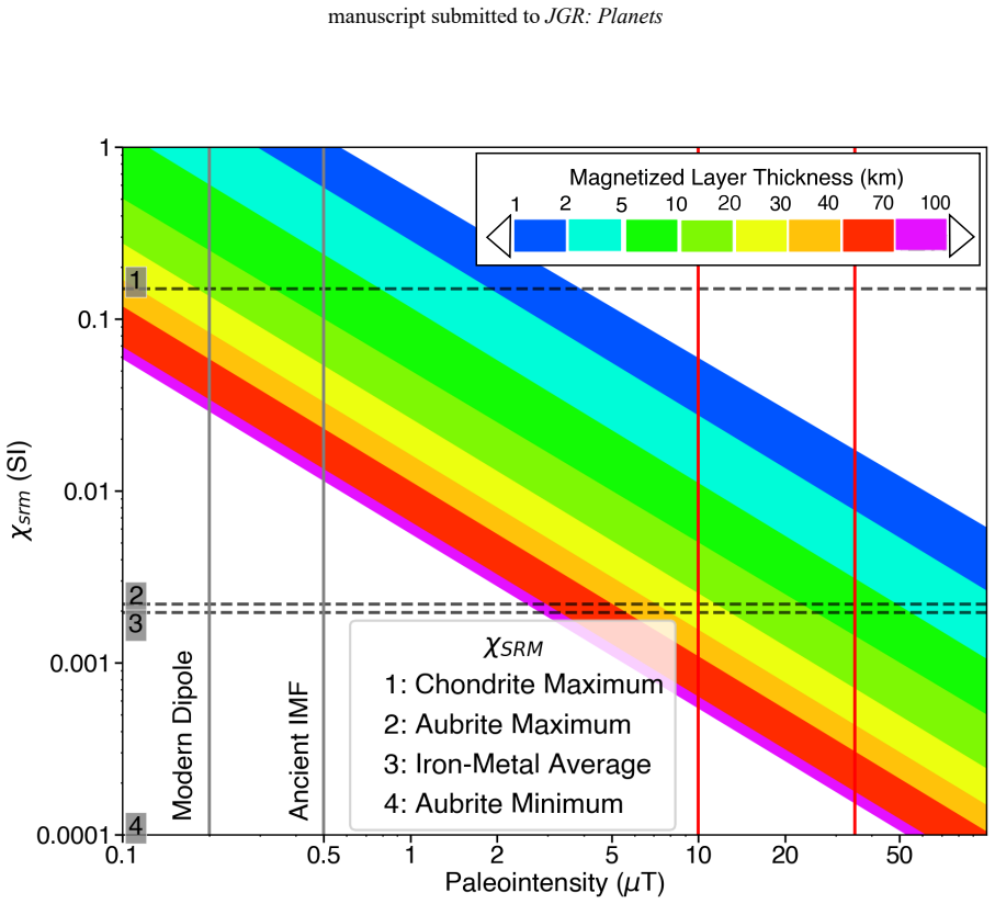
and with 𝜒%"# ≤ 0.1𝜒&"# (Figure 13). The magnetic mineralogy of the Hermean surface is poorly constrained, with measurements of the average crustal (~1.75 wt%) Fe content and compositional features indicating formation in extremely reducing conditions [oxygen fugacity, log fO2, ranging from 3-7 units below the iron-wüstite buffer, (Zolotov et al., 2013)]....
work page 2013
-
[8]
at the time of the Caloris impact (i.e., ~2 μT), the amplified field would have been ~34 μT and could explain these crustal signals with Fe-metal in a magnetized layer just ~7-km thick. As mentioned previously, the Caloris antipode region is found within the H-11 Discovery Quadrangle (22°S-65°S and 270°E- manuscript submitted to JGR: Planets 360°E), which...
work page 1988
-
[9]
and is antipodal to a region of weaker ~5-10 nT crustal fields [Figure 6.19 in (Johnson et al., 2018)] that is not co-located with the Caloris-aged effusive volcanism. It is possible that these weak crustal magnetic field signals antipodal to the Rembrandt basin could be (partially) produced by SRM recorded during the impact plasma amplification of the He...
work page 2018
-
[10]
of large basin antipodes (e.g., Caloris, Rembrandt, Andal-Coleridge, Matisse-Repin, Eitkou-Milton, and Sadi-Scopus) could provide information on the source field and process for magnetizing the surface, which in turn could help place a relative age (compared to the impact event). For example, high surface resolution measurements of the crustal fields anti...
-
[11]
https://doi.org/10.1029/2001JA009217 manuscript submitted to JGR: Planets Caciagli, A., Baars, R
Journal of Geophysical Research: Space Physics, 107(A11), SSH 20-21–SSH 20-11. https://doi.org/10.1029/2001JA009217 manuscript submitted to JGR: Planets Caciagli, A., Baars, R. J., Philipse, A. P., & Kuipers, B. W. M. (2018). Exact expression for the magnetic field of a finite cylinder with arbitrary uniform magnetization. Journal of Magnetism and Magneti...
-
[12]
https://doi.org/10.1051/0004-6361/201525660 Galluzzi, V ., Oliveira, J. S., Wright, J., Rothery, D. A., & Hood, L. L. (2021). Asymmetric Magnetic Anomalies Over Young Impact Craters on Mercury. Geophysical Research Letters, 48(5), e2020GL091767. https://doi.org/10.1029/2020GL091767 Glassmeier, K.-H., Grosser, J., Auster, U., Constantinescu, D., Narita, Y ...
-
[13]
https://doi.org/10.12942/lrsp-2007-3 Heyner, D., Auster, H. U., Fornaçon, K. H., Carr, C., Richter, I., Mieth, J. Z. D., Exner, W., Motschmann, U., Baumjohann, W., Matsuoka, A., Magnes, W., Berghofer, G., Fischer, D., Plaschke, F., Nakamura, R., Narita, Y ., Delva, M., V olwerk, M., … Glassmeier, K. H. (2021). The BepiColombo planetary magnetometer MPO-MA...
-
[14]
https://doi.org/10.1088/0004-637X/750/2/133 Hood, L. L. (1987). Magnetic field and remanent magnetization effects of basin-forming impacts on the Moon. Geophysical Research Letters, 14(8), 844–847. https://doi.org/10.1029/GL014i008p00844 manuscript submitted to JGR: Planets Hood, L. L. (2015). Initial mapping of Mercury's crustal magnetic field: Relations...
-
[15]
P., Güdel, M., Brott, I., & Lüftinger, T
https://doi.org/10.1051/0004-6361/201629609 Johnstone, C. P., Güdel, M., Brott, I., & Lüftinger, T. (2015). Stellar winds on the main-sequence. Astronomy & Astrophysics,
-
[16]
https://doi.org/10.1051/0004-6361/201425301 Kalski, R., Plattner, A. M., Johnson, C. L., & Crane, K. T. (2025). Crustal magnetization source depths north of the Caloris basin, Mercury. Geophysical Research Letters, 52(7), e2024GL114444, https://doi.org/https://doi.org/10.1029/2024GL114444 Kletetschka, G., Fuller, M. D., Kohout, T., Wasilewski, P. J., Herr...
-
[17]
https://doi.org/10.1051/0004-6361/202450177 Murray, B. C., Belton, M. J., Danielson, G. E., Davies, M. E., Gault, D. E., Hapke, B., O'Leary, B., Strom, R. G., Suomi, V ., & Trask, N. (1974). Mercury's surface: Preliminary description and interpretation from Mariner 10 pictures. Science, 185(4146), 169-179. https://doi.org/10.1126/science.185.4146.169 Narr...
-
[18]
Meteoritics & Planetary Science, 44(3), 405-427
Achondrites. Meteoritics & Planetary Science, 44(3), 405-427. https://doi.org/10.1111/j.1945-5100.2009.tb00741.x Rodriguez, J. A. P., Leonard, G. J., Kargel, J. S., Domingue, D., Berman, D. C., Banks, M., Zarroca, M., Linares, R., Marchi, S., Baker, V . R., Webster, K. D., & Sykes, M. (2020). The chaotic terrains of Mercury reveal a history of planetary v...
-
[19]
https://doi.org/10.1038/s41598-020-59885-5 Rothery, D. A., Massironi, M., Alemanno, G., Barraud, O., Besse, S., Bott, N., Brunetto, R., Bunce, E., Byrne, P., Capaccioni, F., Capria, M. T., Carli, C., Charlier, B., Cornet, T., Cremonese, G., D’Amore, M., De Sanctis, M. C., Doressoundiram, A., Ferranti, L., … Zambon, F. (2020). Rationale for BepiColombo stu...
-
[20]
https://doi.org/10.1007/s11214-020-00694-7 manuscript submitted to JGR: Planets Schield, M. A. (1969). Pressure balance between solar wind and magnetosphere. Journal of Geophysical Research, 74(5), 1275-1286. https://doi.org/10.1029/JA074i005p01275 Schultz, P. H., & Gault, D. E. (1975). Seismic effects from major basin formations on the moon and mercury. ...
-
[21]
https://doi.org/10.1007/s41116-021-00029-w Vidotto, A. A., Gregory, S. G., Jardine, M., Donati, J. F., Petit, P., Morin, J., Folsom, C. P., Bouvier, J., Cameron, A. C., Hussain, G., Marsden, S., Waite, I. A., Fares, R., Jeffers, S., & do Nascimento, J. D. (2014). Stellar magnetism: empirical trends with age and rotation. Monthly manuscript submitted to JG...
-
[22]
https://doi.org/10.1038/s41467-021-26860-1 Wang, Y ., Xiao, Z., Chang, Y ., Xu, R., & Cui, J. (2021). Short‐term and global‐wide effusive volcanism on Mercury around 3.7 Ga. Geophysical Research Letters, 48(20), e2021GL094503. https://doi.org/10.1029/2021gl094503 Watters, T. R., Cook, A. C., & Robinson, M. S. (2001) Large-scale lobate scarps in the southe...
-
[23]
Antipodal surface normal unit vector given by 𝒏,$
Dipole center is (0,0,0.2) RM with equatorial strength 2000 nT (dipole moment ~3×10¹⁹ Am2). Antipodal surface normal unit vector given by 𝒏,$. Table 1: Impact plasma simulation cases parameter space. Columns list (left) simulation case, (middle) IMF vector components, BIMF, in nT, and (right) notes on the design of the case, impact geometry, and dipole fi...
work page 2000
-
[24]
and magnetic field relaxation, respectively. The left column shows the evolution of the (log-scale) plasma mass density, 𝜌, with velocity flow direction (white arrows). The middle column shows the evolution of the total magnetic field magnitude normalized to the 0.5 μT IMF, 𝐵/𝐵IMF,0, with magnetic field direction (black arrows). The right column shows a c...
work page 2011
-
[25]
The impact is launched from (X = -0.866, Z = 0.5 RM). manuscript submitted to JGR: Planets Figure 7: Amplification of the IMF and Hermean dynamo field by a Caloris-sized impact at ~30°N when the IMF is parallel and anti-parallel to the impact antipode normal (Cases 4 and 4-Reverse). 2D slices of the 3D-MHD simulation of impact plasma expanding from ~30°N ...
work page 2011
-
[26]
and magnetic field relaxation, respectively. The left column shows the evolution of the (log-scale) plasma mass density, 𝜌, with velocity flow direction (white arrows). The middle and right columns show the evolution of the total magnetic field magnitude normalized to the 0.5 μT IMF, 𝐵/𝐵IMF,0, with magnetic field direction (black arrows) in the X-Z and Y-...
work page 2011
-
[27]
and magnetic field relaxation, respectively. The left column shows the evolution of the (log-scale) plasma mass density, 𝜌, with velocity flow direction (white arrows). The middle column shows the evolution of the total magnetic field magnitude normalized to the 2 μT equatorial dipole field, 𝐵/𝐵dip,0, with magnetic field direction (black arrows). The righ...
work page 2011
-
[28]
maximized antipodal magnetic field due to the compression of anti-parallel and parallel magnetic field, respectively. Cases 3, 4, 4-Reverse, and 5 account for the Caloris impact location and the modern shifted dipole-center, resulting in similar amplified magnetic fields of ~10-14 μT that occur between 35 and 40 minutes. Case 6 shows a heightened final am...
work page 1977
-
[29]
manuscript submitted to JGR: Planets Figure 13: Shock remanent magnetization efficiency, paleointensity, and layer thickness of magnetized materials that can produce 5 nT crustal anomalies. Thicknesses (color bar) required to magnetize crustal material and generate a 5 nT field observed at 20-km altitude for varying ambient, ancient magnetic fields (paleo...
work page 2018
-
[30]
for possible native Hermean material (aubrite-like or iron-metal) and non-native, impact delivered materials (chondritic composition) representing an upper limit with 𝜒%"# = 0.1𝜒&"#, in line with the SRM experiments of (Tikoo et al., 2015). The grey vertical lines represent the initial magnetic field strengths, with the leftmost being the 0.2 μT dipole fi...
work page 2015
discussion (0)
Sign in with ORCID, Apple, or X to comment. Anyone can read and Pith papers without signing in.