Long-time behaviour of sphalerons in φ⁴ models with a false vacuum
Pith reviewed 2026-05-18 09:56 UTC · model grok-4.3
The pith
A growing perturbation turns a sphaleron into an accelerating kink-antikink pair whose fronts approach light speed.
A machine-rendered reading of the paper's core claim, the machinery that carries it, and where it could break.
Core claim
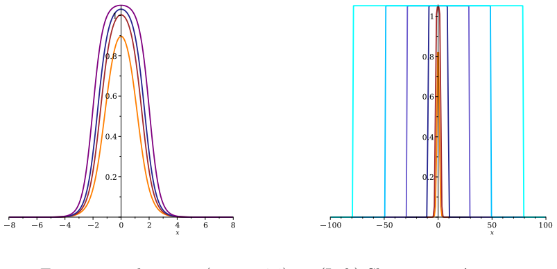
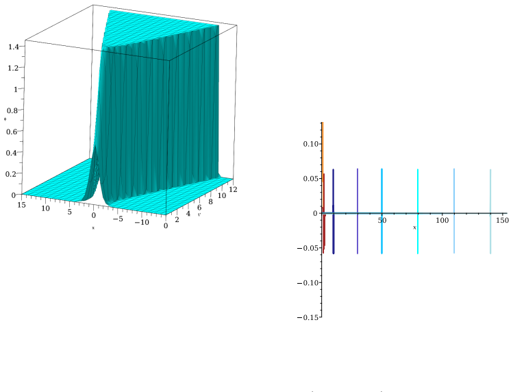
Numerical simulations show the sphaleron evolving into an accelerating kink-antikink pair whose separation increases in time and asymptotically approaches the speed of light. The nonlinear collective coordinate method with three dynamical parameters yields an explicit asymptotic solution describing a spreading tabletop profile whose height approaches the true vacuum while its flanks steepen and accelerate outward. In addition, the energy density concentrates at the flanks, indicating the onset of a gradient blow-up at large times.
What carries the argument
The nonlinear collective coordinate method with three dynamical parameters, which reduces the field dynamics to ordinary differential equations and permits a power-series asymptotic analysis of the late-time spreading profile.
If this is right
- The kink-antikink separation grows continuously and approaches light-speed separation at late times.
- The central region of the field configuration flattens and approaches the true vacuum value.
- The outward flanks accelerate and steepen while carrying most of the energy density.
- The overall structure expands without bound, providing an explicit example of relativistically expanding fronts in nonlinear scalar theories.
Where Pith is reading between the lines
- The same late-time mechanism may govern the expansion of near-sphaleron configurations in other scalar models that possess a false vacuum.
- The predicted concentration of gradients at the fronts could be examined by adding small dissipative or higher-order derivative terms to test regularization.
- Coupling the model to gravity or to additional fields might change the terminal speed reached by the accelerating flanks.
Load-bearing premise
The three-parameter collective coordinate ansatz remains a faithful reduced description of the full field dynamics at arbitrarily late times, even after the fronts have become relativistic and the energy has concentrated at the flanks.
What would settle it
A high-resolution numerical evolution of the original partial differential equation to much later times that measures whether the maximum field gradient at the fronts continues to increase without bound or saturates at a finite value.
Figures


read the original abstract
Evolution of sphalerons in a class of quartic Klein-Gordon models are studied under a growing perturbation. Sphalerons are unstable lump-like solutions that arise from a saddle point between true and false vacua in the energy functional. Numerical simulations are presented which show the sphaleron evolving into an accelerating kink-antikink pair whose separation increases in time and asymptotically approaches the speed of light. To explain this behaviour analytically, a nonlinear collective coordinate method is developed which has three dynamical parameters and leads to an explicit asymptotic solution using a power series expansion. The solution describes the emergence of a spreading tabletop profile whose height approaches the true vacuum while its flanks steepen and accelerate outward. In addition, the energy density is shown to concentrate at the flanks, indicating the onset of a gradient blow-up at large times. These results provide a detailed description of the long-time dynamics of positively perturbed sphalerons, and reveal a universal mechanism for the formation of relativistically expanding structures in nonlinear field theories.
Editorial analysis
A structured set of objections, weighed in public.
Referee Report
Summary. The manuscript examines the long-time evolution of sphalerons in quartic Klein-Gordon models with a false vacuum. Numerical simulations show a positively perturbed sphaleron developing into an accelerating kink-antikink pair whose separation grows and asymptotically approaches the speed of light. A nonlinear collective-coordinate reduction with three dynamical parameters is introduced; its equations are derived from the field equation and solved via power-series expansion to obtain an explicit asymptotic solution describing a spreading tabletop profile whose height approaches the true vacuum, with steepening flanks that accelerate outward and with energy density concentrating at the flanks, indicating the onset of gradient blow-up.
Significance. If the central claims hold, the work supplies both numerical evidence and an explicit analytic asymptotic description of sphaleron instability leading to relativistically expanding structures. The combination of a three-parameter collective-coordinate ansatz with a power-series solution is a constructive approach that yields concrete predictions for the late-time profile and energy localization; these features could prove useful for understanding analogous phenomena in other nonlinear field theories.
major comments (1)
- [Collective coordinate reduction and asymptotic expansion] The validity of the three-parameter collective-coordinate ansatz at arbitrarily late times is load-bearing for the explicit asymptotic solution and the claims of height approaching the true vacuum and gradient blow-up. Once the fronts become relativistic and energy concentrates at the steepening flanks (as reported in the numerical simulations), it is not demonstrated that radiation or modes orthogonal to the ansatz remain negligible. A direct comparison of the reduced dynamics against the full Klein-Gordon evolution at large times, or an estimate of the projection onto orthogonal modes, would be required to substantiate that the power-series solution remains faithful.
minor comments (2)
- The abstract states that the separation 'asymptotically approaches the speed of light' but does not specify the precise functional form (e.g., 1 - v ~ t^α) obtained from the power series; adding this would improve clarity.
- Notation for the three collective coordinates and the potential parameters should be introduced with a single consistent table or list early in the text to aid readability.
Simulated Author's Rebuttal
We thank the referee for the careful reading and constructive comments on our manuscript. We address the major comment below and are prepared to revise the paper accordingly to strengthen the substantiation of the collective-coordinate results.
read point-by-point responses
-
Referee: The validity of the three-parameter collective-coordinate ansatz at arbitrarily late times is load-bearing for the explicit asymptotic solution and the claims of height approaching the true vacuum and gradient blow-up. Once the fronts become relativistic and energy concentrates at the steepening flanks (as reported in the numerical simulations), it is not demonstrated that radiation or modes orthogonal to the ansatz remain negligible. A direct comparison of the reduced dynamics against the full Klein-Gordon evolution at large times, or an estimate of the projection onto orthogonal modes, would be required to substantiate that the power-series solution remains faithful.
Authors: We thank the referee for identifying this key point. The three-parameter ansatz was constructed precisely to encode the dominant late-time features seen in the full numerical evolution: the tabletop height approaching the true vacuum, the outward acceleration of the flanks, and the concentration of energy density there. To address concerns about orthogonal modes and radiation, we will add a new subsection that directly compares the collective-coordinate solution against the full Klein-Gordon field evolution at progressively later times, including regimes where the fronts are relativistic. We will also include a quantitative estimate of the projection of the numerical solutions onto the subspace orthogonal to the ansatz, obtained by decomposing the simulated field configurations. These additions will show that deviations remain small up to the times accessible in our simulations and that the power-series asymptotic form continues to capture the leading behavior. We agree that such evidence is necessary to support the claims and will incorporate it in the revised manuscript. revision: yes
Circularity Check
No significant circularity: reduced dynamics derived from field equation projection, not forced by fit or self-citation
full rationale
The paper presents independent numerical simulations of the full Klein-Gordon dynamics showing the sphaleron evolving into an accelerating kink-antikink pair. It then introduces a three-parameter collective coordinate ansatz and derives the reduced ODEs by projecting the field equation onto the ansatz manifold. The asymptotic power-series solution is obtained directly from those reduced equations. This is a standard variational reduction whose output is not equivalent to its inputs by construction, nor does it rely on self-citation chains or renaming of known results. The assumption that the ansatz remains accurate at late times is a modeling limitation affecting correctness, not a circularity in the derivation chain itself.
Axiom & Free-Parameter Ledger
free parameters (1)
- three collective coordinates
axioms (1)
- domain assumption The field equation is the quartic Klein-Gordon equation with a double-well potential possessing a false vacuum.
Forward citations
Cited by 1 Pith paper
-
Collision Dynamics of False-Vacuum Oscillons
Oscillon collisions in false-vacuum scalar theories produce reflection, crossing, resonance windows, and can initiate true-vacuum phase transitions when energy suffices.
Reference graph
Works this paper leans on
-
[1]
Y.M. Shnir,Topological and Non-Topological Solitons in Scalar Field Theories, Cambridge University Press, Cambridge U.K., 2018
work page 2018
-
[2]
Manton, The inevitability of sphalerons in field theory, Phil
N.S. Manton, The inevitability of sphalerons in field theory, Phil. Trans. R. Soc. A 377 (2019), 20180327
work page 2019
- [3]
-
[4]
Yaffe, Static solutions of SU(2)-Higgs theory, Phys
L.G. Yaffe, Static solutions of SU(2)-Higgs theory, Phys. Rev. D 40(10) (1989), 3463–3473
work page 1989
-
[5]
Klinkhamer, A new sphaleron in the Weinberg-Salam theory, Phys
F.R. Klinkhamer, A new sphaleron in the Weinberg-Salam theory, Phys. Lett. B 246 (1990), 131–134
work page 1990
- [6]
- [7]
-
[8]
Y. Shnir, D.H. Tchrakian, Axially-symmetric sphaleron solutions of the Skyrme model, J. Phys. Conf. Ser. 284 (2011), 012053
work page 2011
- [9]
-
[10]
F.R. Klinkhamer, N.S. Manton, A saddle point solution in the Weinberg-Salam theory, Phys. Rev. D 30 (1984), 2212–2220
work page 1984
- [11]
- [12]
-
[13]
C. Adam, D. Ciurla, K. Oles, T. Romanczukiewicz, A. Wereszczynski, Sphalerons and resonance phe- nomenon in kink-antikink collisions, Phys. Rev. D 104 (2021), 105022
work page 2021
-
[14]
K. Oles, J. Queiruga, T. Romanczukiewicz, A. Wereszczynski, Sphaleron without shape mode and its oscillon, Phys. Lett. B 847 (2023), 138300
work page 2023
-
[15]
A. Alonso-Izquierdo, S. Navarro-Obrego´ n, K. Oles, J. Queiruga, T. Romanczukiewicz, A. Wereszczynski, Semi-Bogomol’nyi-Prasad-Sommerfield sphaleron and its dynamics, Phys. Rev. E 108 (2023), 064208
work page 2023
- [16]
-
[17]
Manton, Integration theory for kinks and sphalerons in one dimension, J
N.S. Manton, Integration theory for kinks and sphalerons in one dimension, J. Phys. A: Math. Theor. 57 (2024), 025202. 30
work page 2024
-
[18]
I.L. Bogolyubsky and V.G. Makhankov, Lifetime of pulsating solitons in certain classical models, JETP Lett. 24 (1976), 12–14
work page 1976
-
[19]
Gleiser, Pseudo-Stable Bubbles, Phys
M. Gleiser, Pseudo-Stable Bubbles, Phys. Rev. D 49 (1994), 2978–2981
work page 1994
-
[20]
M. Gleiser and D. Sicilia, General theory of oscillon dynamics, Phys. Rev. D 80 (2009), 125037
work page 2009
-
[21]
S. Navarro-Obrego´ n, J. Queiruga, Impact of the internal modes on the sphaleron decay, Eur. Phys. J. C (2024) 84:821
work page 2024
-
[22]
Anco, Instability of sphalerons inϕ 4 models with a false vacuum
S.C. Anco, Instability of sphalerons inϕ 4 models with a false vacuum. arxiv: 2508.12150
-
[23]
Ronveaux (ed.),Heun’s Differential Equation, Oxford University Press, 1995
A. Ronveaux (ed.),Heun’s Differential Equation, Oxford University Press, 1995
work page 1995
-
[24]
A. Geyer, D.E. Pelinovsky,Stability of nonlinear waves in Hamiltonian dynamical systems, American Mathematical Society, Providence RI, 2025
work page 2025
- [25]
discussion (0)
Sign in with ORCID, Apple, or X to comment. Anyone can read and Pith papers without signing in.