Sub-exponential Growth Dynamics in Complex Systems: A Piecewise Power-Law Model for the Diffusion of New Words and Names
Pith reviewed 2026-05-22 13:06 UTC · model grok-4.3
The pith
A piecewise power-law model shows that sub-exponential growth with shape parameter near 0.5 describes most diffusion of new words and names.
A machine-rendered reading of the paper's core claim, the machinery that carries it, and where it could break.
Core claim
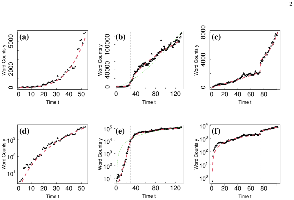
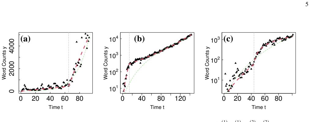
The central discovery is that sub-exponential growth is a common pattern in social diffusion of new words and names, as evidenced by the mode of the shape parameter alpha being near 0.5 in single-segment fits, and that 55% of selected patterns without abrupt shifts are adequately described by one or two segments of the piecewise power-law model, with peak scale mainly determined by the growth rate R.
What carries the argument
The piecewise power-law model, which fits growth curves using segments of the form proportional to t to the power alpha, with parameters for growth rate R, shape alpha, and duration T per segment.
If this is right
- Single-segment diffusion curves have a mode of alpha near 0.5, showing sub-exponential growth prevails.
- The peak diffusion scale depends primarily on the growth rate R rather than alpha or duration T.
- Alpha tends to be smaller for niche or local topics and larger for widely shared ones.
- Alpha serves as an index of preference for outward-oriented communication in a micro-behavioral model.
Where Pith is reading between the lines
- Applying this model to epidemic spread or technology adoption could reveal similar sub-exponential patterns in other complex systems.
- If alpha measures outward communication preference, then social network structures might predict or influence alpha values in diffusion.
- The results suggest revising predictive models for idea spread to account for sub-exponential rather than exponential early phases.
- Cross-platform comparisons could test whether the 55% fit rate and alpha distribution hold in non-Japanese data.
Load-bearing premise
The selection of 2,963 items based on sufficient duration, peak, and monotonic growth yields a sample whose alpha distribution and segment numbers apply to broader diffusion processes.
What would settle it
Observing that the distribution of fitted alpha values in a new large dataset of word diffusions peaks significantly away from 0.5 or that most curves need more than two segments to fit well would falsify the prevalence of this sub-exponential pattern.
Figures


read the original abstract
The diffusion of ideas and language in society has conventionally been described by S-shaped models, such as the logistic curve. However, the role of sub-exponential growth -- a slower-than-exponential pattern known in epidemiology -- has been largely overlooked in broader social phenomena. Here, we present a piecewise power-law model to characterize complex growth curves with a few parameters. We systematically analyzed a large-scale dataset of approximately one billion Japanese blog articles linked to Wikipedia vocabulary, and observed consistent patterns in web search trend data (English, Spanish, and Japanese). Our analysis of 2,963 items, selected for reliable estimation (e.g., sufficient duration/peak, monotonic growth), reveals that 1,625 (55%) diffusion patterns without abrupt level shifts were adequately described by one or two segments. For single-segment curves, we found that (i) the mode of the shape parameter $\alpha$ was near 0.5, indicating prevalent sub-exponential growth; (ii) the peak diffusion scale is primarily determined by the growth rate $R$, with minor contributions from $\alpha$ or the duration $T$; and (iii) $\alpha$ showed a tendency to vary with the nature of the topic, being smaller for niche/local topics and larger for widely shared ones. Furthermore, a micro-behavioral model of outward (stranger) vs. inward (community) contact suggests that $\alpha$ can be interpreted as an index of the preference for outward-oriented communication. These findings suggest that sub-exponential growth is a common pattern of social diffusion, and our model provides a practical framework for consistently describing, comparing, and interpreting complex and diverse growth curves.
Editorial analysis
A structured set of objections, weighed in public.
Referee Report
Summary. The paper introduces a piecewise power-law model for characterizing the diffusion of new words and names in complex social systems. Using a large dataset of approximately one billion Japanese blog articles linked to Wikipedia vocabulary, along with web search trend data in English, Spanish, and Japanese, the authors analyze 2,963 selected items that meet criteria for reliable estimation including sufficient duration/peak and monotonic growth. They report that 1,625 (55%) of diffusion patterns without abrupt level shifts are adequately described by one or two power-law segments. For single-segment curves, the mode of the shape parameter α is near 0.5, suggesting prevalent sub-exponential growth. The peak diffusion scale is primarily determined by the growth rate R, with α varying by topic nature (smaller for niche topics). A micro-behavioral model interprets α as an index of preference for outward-oriented communication.
Significance. If the central empirical findings hold, this work would be significant for social physics and diffusion studies by demonstrating that sub-exponential growth, rather than purely S-shaped logistic patterns, is a common feature in the spread of ideas and language. The piecewise power-law approach offers a practical, few-parameter framework for describing and comparing diverse growth curves. Strengths include the scale of the dataset (~1 billion articles) and validation across multiple languages. The interpretation linking α to communication preferences provides a micro-foundation, though it remains suggestive.
major comments (3)
- The abstract states that items were selected for 'reliable estimation (e.g., sufficient duration/peak, monotonic growth)'. This filter, particularly the monotonic growth requirement, risks biasing the sample toward sub-exponential patterns by excluding non-monotonic, abrupt-shift, or super-exponential trajectories. No statistics on the excluded items or sensitivity analyses relaxing the monotonicity criterion while retaining other thresholds are reported, which is load-bearing for the claim that 55% of patterns are described by one or two segments and that α mode is near 0.5.
- The abstract reports specific results such as 55% (1,625 items), modal α near 0.5, and dominance of R over α and T in determining peak scale, yet no details are provided on the fitting algorithm used for the power-law segments, uncertainty quantification (e.g., confidence intervals on α), or comparisons to alternative models like logistic curves. This absence undermines the robustness of the quantitative claims.
- The micro-behavioral model suggesting that α indexes preference for outward (stranger) vs. inward (community) contact is offered as an interpretive framework rather than a derivation that predicts or recovers the observed distribution of α values from the data. This leaves the connection between the fitted parameter and the behavioral mechanism qualitative.
minor comments (1)
- The claim of 'consistent patterns' in web search trend data across languages would benefit from specifying the number of items analyzed in each language and the quantitative measure of consistency used.
Simulated Author's Rebuttal
We thank the referee for their constructive and detailed comments. These have highlighted important areas for improving methodological transparency and addressing potential selection effects. We provide point-by-point responses below and will revise the manuscript accordingly.
read point-by-point responses
-
Referee: The abstract states that items were selected for 'reliable estimation (e.g., sufficient duration/peak, monotonic growth)'. This filter, particularly the monotonic growth requirement, risks biasing the sample toward sub-exponential patterns by excluding non-monotonic, abrupt-shift, or super-exponential trajectories. No statistics on the excluded items or sensitivity analyses relaxing the monotonicity criterion while retaining other thresholds are reported, which is load-bearing for the claim that 55% of patterns are described by one or two segments and that α mode is near 0.5.
Authors: We agree that the monotonic growth filter could introduce bias toward certain growth patterns and that the lack of information on excluded items limits assessment of robustness. In the revised manuscript we will report the number and basic characteristics of items excluded by each criterion (including non-monotonicity and abrupt shifts). We will also add sensitivity analyses that relax the monotonicity requirement while keeping other selection thresholds and show how the reported 55% figure and the mode of α change under these relaxed conditions. revision: yes
-
Referee: The abstract reports specific results such as 55% (1,625 items), modal α near 0.5, and dominance of R over α and T in determining peak scale, yet no details are provided on the fitting algorithm used for the power-law segments, uncertainty quantification (e.g., confidence intervals on α), or comparisons to alternative models like logistic curves. This absence undermines the robustness of the quantitative claims.
Authors: We accept that additional methodological detail is required to support the quantitative results. The revised manuscript will include a full description of the segment-fitting procedure, the optimization method, and the criteria used to decide between one and two segments. We will also report uncertainty estimates (e.g., bootstrap confidence intervals) for the fitted α values. Finally, we will add direct comparisons with logistic growth models using standard model-selection metrics such as AIC and residual diagnostics. revision: yes
-
Referee: The micro-behavioral model suggesting that α indexes preference for outward (stranger) vs. inward (community) contact is offered as an interpretive framework rather than a derivation that predicts or recovers the observed distribution of α values from the data. This leaves the connection between the fitted parameter and the behavioral mechanism qualitative.
Authors: We acknowledge that the micro-behavioral model is presented as an interpretive framework and does not constitute a quantitative derivation that recovers the empirical distribution of α. In the revision we will explicitly state its qualitative nature, clarify the assumptions involved, and note that stronger empirical tests would require additional contact-pattern data. We believe the framework still offers useful conceptual insight but agree it remains suggestive rather than predictive. revision: partial
Circularity Check
No significant circularity: empirical fitting and observational reporting
full rationale
The paper proposes a piecewise power-law model as a descriptive tool and applies it to a filtered dataset of 2,963 items meeting explicit criteria (sufficient duration/peak and monotonic growth). Reported results such as the 55% one/two-segment fraction and single-segment alpha mode near 0.5 are direct outputs of parameter fitting to the selected observations, not predictions or derivations that reduce to the model inputs by construction. The micro-behavioral interpretation of alpha as an outward-contact index is presented as a suggestive framework rather than a closed-form recovery of the fitted values. No self-citations, uniqueness theorems, ansatzes smuggled via prior work, or self-definitional equations appear in the provided sections. The analysis remains self-contained as an empirical characterization study with transparent selection rules.
Axiom & Free-Parameter Ledger
free parameters (3)
- alpha =
mode near 0.5
- R
- T
axioms (1)
- domain assumption Monotonic diffusion curves without abrupt level shifts can be adequately approximated by one or two power-law segments.
Lean theorems connected to this paper
-
IndisputableMonolith/Cost/FunctionalEquation.leanwashburn_uniqueness_aczel (J uniquely satisfies the calibrated reciprocal functional equation) echoes?
echoesECHOES: this paper passage has the same mathematical shape or conceptual pattern as the Recognition theorem, but is not a direct formal dependency.
dy_i(t)/dt = R_i Y (y_i(t)/Y)^α_i (Eq. 1); solution s(τ) = ((1-α)τ + 1)^{1/(1-α)} for α ≠ 1
-
IndisputableMonolith/Foundation/AlphaCoordinateFixation.leanalpha_pin_under_high_calibration (higher-derivative calibration forces α = 1) contradicts?
contradictsCONTRADICTS: the theorem conflicts with this paper passage, or marks a claim that would need revision before publication.
α_i = 1 - γ_i / Q (behavioral derivation, Eq. 11)
What do these tags mean?
- matches
- The paper's claim is directly supported by a theorem in the formal canon.
- supports
- The theorem supports part of the paper's argument, but the paper may add assumptions or extra steps.
- extends
- The paper goes beyond the formal theorem; the theorem is a base layer rather than the whole result.
- uses
- The paper appears to rely on the theorem as machinery.
- contradicts
- The paper's claim conflicts with a theorem or certificate in the canon.
- unclear
- Pith found a possible connection, but the passage is too broad, indirect, or ambiguous to say the theorem truly supports the claim.
Reference graph
Works this paper leans on
-
[1]
Japanese Blog Data We obtain daily word-appearance counts from a nation- wide corpus of Japanese blogs using the large-scale database “Kuchikomi@kakaricho,” provided by Hottolink, Inc. The database contains approximately nine billion blog articles and covers about 90% of Japanese blogs over the period from November 1, 2006 to December 31, 2019 [32]. a. Bo...
work page 2006
-
[2]
We use it in parallel with blog post counts to quantify social interest (see the red circles in Fig
Google Trends Google Trends provides a monthly index of search volume for a given query term on the Google search engine [33]. We use it in parallel with blog post counts to quantify social interest (see the red circles in Fig. S1). The series is normalized by Google so that the maximum value within the observation window equals 100, with other values sca...
work page 2015
-
[3]
Blog Data We extracted candidate words in two steps
-
[4]
From the list of article titles in the Japanese edition of Wikipedia [34], we identified the one million titles that occurred most frequently in our Japanese blog corpus
-
[5]
From these one million titles, we selected 20,764 titles that had zero blog posts in both November and December 2006
work page 2006
-
[6]
Google Trends For the Google Trends analysis, we used Wikipedia page views to preselect newly emerging words in each of the English, Spanish, and Japanese editions of Wikipedia [34]
-
[7]
We collected page-view counts for the first day of each month from May 2015 through January 2022
work page 2015
-
[8]
We defined a “new word” as a title with zero page views on May 1, 2015 (the first observation month) and with at least 50 page views for Spanish or at least 1,000 page views for English on January 1 of any year from 2016 to 2022. For Japanese, we used the same 20,764-word dictionary as in the blog data
work page 2015
-
[9]
For titles meeting this criterion, we retrieved Google Trends time series via the Google Trends API [33]. Appendix D3: Normalization of Word-Count Time Series for Blog Data We define notation for the word-count series𝑥 𝑖 (𝑡)and the normalized series𝑦 𝑖 (𝑡)as follows [20]. •The time step is set to 30 days. When𝑡increases by one, real time advances by 30 da...
-
[10]
However, in this study, we add a further correction using the method in the next Section 2
Extracting the Beginning of Growth The extraction of the growth starting point basically follows the procedure shown in [20]. However, in this study, we add a further correction using the method in the next Section 2. Prior to the correction in Section 2, the procedure based on
-
[11]
(the procedure to determine a provisional starting point) is shown below. 1.Calculate the upper limit for candidates,𝑇 𝑠.This upper limit is set as the time when the 13-point moving median first reaches the 25th percentile point:𝑇 𝑠 = min𝑡 {𝑡|𝑦 𝑗 (𝑡) ≥Quantile 0.25{𝑦 𝑗 (𝑡)}}. This procedure is introduced to avoid incorrectly selecting a minimum point duri...
-
[12]
Refining the Start Point by Excluding an Early Low-Level Segment Buried in Noise For the initial time𝑡 𝑠 0 (determined in Section 1), we perform a further investigation and correction in this study. When 𝑦 𝑗 (𝑡)is small, relative fluctuations (e.g., Poisson-like noise) can become large and hide a slow growth component. In such cases, the piecewise growth ...
-
[13]
Extraction of End of Growth The end point of growth follows the method of [20]. We introduce it below. The end point of growth,𝑡 𝑒 0, is basically detected as the point at which a clear downward trend begins. Here, a “clear downward trend” is defined as a point at or after the growth starting point (𝑡 𝑠 0 ≤𝑡 𝑒
-
[14]
from which the word count continu- ously decreases for at least 12 time points (approximately 12 months). As a specific procedure, first, we roughly search for the starting point of the downtrend using the 13-point moving median to avoid being fooled by local trends. Next, we refine the candidate points by progressively using information from smaller time...
-
[15]
This transformed time is𝑡 𝑒 6. 7.Comparing the candidate𝑡 𝑒 6 with the global max- imum point𝑡 𝑚𝑎𝑥 :Finally, we compare the candi- date point𝑡 𝑒 6 obtained from this procedure with the global maximum point of the entire time series,𝑡 𝑚𝑎𝑥 = argmax𝑡 [𝑦 𝑗 (𝑡)]. If𝑡 𝑚𝑎𝑥 exists within 6 points before or after𝑡 𝑒 6 (i.e.,𝑡 𝑒 6 −6≤𝑡 𝑚𝑎𝑥 ≤𝑡 𝑒 6 +6), we check whet...
-
[16]
within the target period. (iii) In a binomial test on the sign of the difference (𝑦 𝑗 (𝑡+1) −𝑦 𝑗 (𝑡)), the proportion of positives (if 𝑡𝑒 6 < 𝑡 𝑚𝑎𝑥 ) or negatives (if𝑡 𝑚𝑎𝑥 < 𝑡 𝑒
-
[17]
is 0.6 or more (one-sided test p-value is less than 5%). If these conditions are met, the final end point is set to 𝑡𝑒 0 =𝑡 𝑚𝑎𝑥 . If the conditions are not met (i.e.,𝑡 𝑚𝑎𝑥 is judged to be a temporary spike), then𝑡 𝑒 0 =𝑡 𝑒 6. Appendix E2: Detecting Large Jumps in the Keyword Frequency Time Series This method is an algorithm to detect when an “abrupt jump”...
-
[18]
, 𝐿), we define the single-segment growth model given by Eq
Defining the Single-Segment Model (𝑁=1) First, for an observed time series𝑦 𝑡 (where𝑡=1, . . . , 𝐿), we define the single-segment growth model given by Eq. 1, ˆ𝑦(𝑡)as follows: ˆ𝑦(𝑡)= 𝑌· n 𝑅· (1−𝛼) (𝑡−𝑡 0) + ˆ𝑦(𝑡0 ) 𝑌 1−𝛼 o1/(1−𝛼) , 𝛼≠1 ˆ𝑦(𝑡0) ·exp 𝑅· (𝑡−𝑡 0) , 𝛼=1 In this model, the parameters we need to estimate are the shape parameter𝛼and theg...
-
[19]
Defining the Final loss function (How We Measure Error) To determine the parameters𝛼and𝑅, we design a ”loss function”L (𝛼, 𝑅)that measures how badly the model fits the data. We then find the parameters that minimize this loss. a. Power Transform and Residuals Before defining the loss function, we first apply a “power transform” to both the observed values...
-
[20]
The Purpose of Our Final Loss Function (Upper-side Robustness) Time series data like keyword frequency (word counts) often have complex noise, especially sudden upward spikes caused by external news. A standard symmetric error measure (like least squares, (𝑦 𝑡 −ˆ𝑦(𝑡))2) would be pulled upward unfairly by these large spikes (outliers). Our loss function is...
-
[21]
Optimization Process The final optimization problem is formulated as finding the arguments that minimize the loss: (ˆ𝛼,ˆ𝑅)=arg min 𝛼∈ [ −10,10],𝑅 𝑟 𝑎𝑤 ∈ [0,10] L (𝛼, 𝑅5 𝑟 𝑎𝑤 ) To ensure𝑅 >0 and stabilize the optimization, we use a search variable𝑅 𝑟 𝑎𝑤 ∈ (0,10]and transform it via𝑅=𝑅 5 𝑟 𝑎𝑤. To solve this global optimization problem, we useDiffer- ential ...
-
[22]
Determination of𝑦(𝑡 0) The initial value ˆ𝑦(𝑡 0)is determined from the smoothed spline ¯𝑦(𝑡)at𝑡 0; if ¯𝑦(𝑡0)<0, we set ˆ𝑦(𝑡 0)=0.8 [20]. Appendix F2: Parameter Estimation for the Piecewise Power-Law Model (𝑁≥2) This section explains how to estimate the parameters for the piecewise power-law model. First, we explain the estimation method for the case with ...
-
[23]
Estimating Split Points for a Fixed𝑁(No Jumps / Continuity Constraint) Here, we describe how to estimate the parameters for the piecewise power-law model when the number of segments𝑁 is already fixed. a. Problem Definition and Objective •Input:A time series with equally spaced points𝑦 𝑡 (from 𝑡=1 to𝑇) and a pre-specified number of segments𝑁 (e.g.,𝑁=2,3,4,...
-
[24]
The final split points are{𝑡 ∗ 1, 𝑡∗ 2}, and the parameters are the ones found in each step. e. Case𝑁=4(Three Split Points) When𝑁=4, we have three split points{𝑡 1, 𝑡2, 𝑡3}. We solve this by splitting the time series into two “𝑁=2 sub-problems”. 1.List candidates for the central split point𝑡 𝑐: We check all𝑡 𝑐 ∈ {3,4, . . . , 𝑇−3}(to leave room for 𝑁=2 sp...
-
[25]
The other splits𝑠 ∗ left and𝑠 ∗ right become𝑡 ∗ 1 and𝑡 ∗
-
[26]
The final set is{𝑡 ∗ 1, 𝑡∗ 2, 𝑡∗ 3}, along with all corresponding parameters. f. Case𝑁≥5(General Recursive Method) For𝑁≥5, we generalize this recursive method. We split the problem into two sub-problems with𝑁 left =⌊𝑁/2⌋segments (left) and𝑁 right =⌈𝑁/2⌉segments (right). 1.List candidates for the central split point𝑡 𝑐: We check all𝑡 𝑐 ∈ {𝑁 left, . . . , 𝑇...
-
[27]
Choosing the Number of Segments𝑁(No Jumps / Continuity Constraint) This section describes the procedure for deciding the seg- ment no𝑁for a keyword-frequency time series𝑦(𝑡). a. Sequential Selection Procedure We assume that the models being compared (the𝑁-segment model and the𝑁+1-segment model) have each already been optimized (i.e., their total loss has ...
-
[28]
split point estimation under continuity
Parameter Estimation for the Model Considering Jumps (Discontinuities) a. Overview and Basic Approach This section explains the parameter estimation procedure for the piecewise power-law model, taking into account the jumps (discontinuous change points)detected in Appendix E2. The basic approach is as follows: •Fixing Jump Locations: The jump locations𝜏 𝑏...
work page 2000
-
[29]
First, the difference (error) between the observed data and the model’s theoretical values is measured as the “Error Area”. This is the area between the two curves when the observed data and the model are plotted
-
[30]
Second, the total signal strength of the theoretical model (relative to its baseline) is measured as the“Model Area”
-
[31]
The smaller this ratio, the better the model fits
Finally, the procedure calculates the ratio of the ”Error Area” to the ”Model Area” (which is the normalized error). The smaller this ratio, the better the model fits. Based on this concept, our comprehensive decision consid- ers the following: •Evaluation Scale: We evaluate the area ratio on two scales: thelinear scale(absolute data values) and the logar...
-
[32]
Definition of Evaluation Metrics To make this decision, we first define the specific errors and quantities used to compare the observed datayand each model ˆy(𝑚) (𝑚=1,2). a. Data Preprocessing and Notation •Observed Data:y=(𝑦 1, 𝑦2, . . . , 𝑦𝐿) •Theoretical Model Values: ˆy(𝑚) =(ˆ𝑦(𝑚) 1 , . . . ,ˆ𝑦(𝑚) 𝐿 ) •Smoothed Observed Data: To reduce short-term nois...
-
[33]
Input the observed valuesyinto the inverse function of Model 1,𝑓 −1 1 (𝑦 𝑡 ), to calculate the “predicted time tpred” at which those values𝑦 𝑡 should have occurred
-
[34]
Define the “Time Prediction Error𝐸 𝑡” as the dis- crepancy (mean absolute error) between this predicted timet pred and the actual observation timet true = (1,2, . . . , 𝐿). 𝐸𝑡 =mean(|t pred −t true |) Interpretation: A small𝐸 𝑡 indicates that Model 1 accu- rately captures the relationship between time and value (i.e., “when” a certain value occurs). We ut...
-
[35]
Model Selection Adjudication Procedure Using the metrics defined above, we establish three criteria (Criterion 1, 2, and 3) to adjudicate whether to adopt Model 1 (ˆy(1) ). Criterion 1: Error Ratio Criterion Objective: To confirm that the relative error area ratio of Model 1 (𝑆1) is not “significantly larger” than that of Model 2 (𝑆2). Condition: The area...
-
[36]
Final Adjudication The final decision is made based on the three criteria above. •Adopt Model 1 ( ˆy(1) , the𝑁-segment model) if: At least oneof Criterion 1, Criterion 2, or Criterion 3 is met. (Interpreted as Model 1 being comparable to, or better than, Model 2, or superior in time prediction.) •Adopt Model 2 ( ˆy(2) , the(𝑁+1)-segment model) if: All of ...
-
[37]
Objective The objective of this section is to systematically extract terms𝑤that tend to co-occur with specific types of neologisms. Specifically, we want to identify if a word𝑤tends to co-occur with: (i) Neologisms showingexponential-like growth (𝛼≈1) (ii) Neologisms showinglinear-like growth (𝛼≈0) To do this, we evaluate the monotonic correlation (rank c...
-
[38]
Data and Definitions We define the data and metrics used in this analysis as follows: •Total occurrences of neologism𝑗;N 𝑗: The total word count of neologism𝑗in the entire corpus. •Proximal co-occurrences𝐶 𝑗 (𝑤): The total number of times𝑤was found within a±40 word window around𝑗(in the same document). (Note: Overlapping windows count the same𝑤multiple ti...
-
[39]
proximal co-occurrence index𝑞 𝑗 (𝑤)
Proximal Co-occurrence Index𝑞 𝑗 (𝑤)and Floor Treatment We define the “proximal co-occurrence index𝑞 𝑗 (𝑤)” to measure the strength of co-occurrence: 𝑞 𝑗 (𝑤)= 𝐶 𝑗 (𝑤) N𝑗 This represents the average number of times𝑤appears near𝑗 (within±40 words) per single occurrence of𝑗. It is a density- like value and can be greater than 1. .1. Floor Treatment (Lower Bou...
-
[40]
(This provides a 0.1 margin around the 0 to 1 range.) 2.Sufficient Occurrences: N𝑗 ≥100
Data Used for Correlation Analysis When calculating the correlation for a co-occurring word 𝑤, we limit the analysis to neologisms𝑗that meet all three of the following conditions: 1.Growth Exponent Range: −0.1≤𝛼 𝑗 ≤1.1. (This provides a 0.1 margin around the 0 to 1 range.) 2.Sufficient Occurrences: N𝑗 ≥100. (We exclude low-frequency neologisms, as their𝑞 ...
-
[41]
Correlation Calculation and Statistics Using the set of neologismsS 𝑤 (sample size𝑛(𝑤)), we calculateKendall’s rank correlation (𝜏)between the floor- treated index𝑞 ⟨0.01⟩ 𝑗 (𝑤)and the growth exponent𝛼 𝑗. (𝜏(𝑤), 𝑝(𝑤))=Kendall 𝑞 ⟨0.01⟩ 𝑗 (𝑤), 𝛼 𝑗 52 •𝜏(𝑤)>0(Positive Correlation): A larger𝑞 𝑗 (𝑤)(co-occurs easily with𝑤) is associ- ated with a larger𝛼 𝑗 (mor...
-
[42]
Criteria for Extracting Co-occurring Terms The co-occurring terms𝑤listed in Table II are those that met the followingReliability Criteriaand one of the two Correlation Strength Criteria. •Reliability Criteria (Scale and Significance): All ex- tracted terms must first meet all of the following condi- tions: –0< 𝑝(𝑤) ≤0.05 (Statistically significant) –𝑛(𝑤) ...
-
[43]
Reference Data (Information Provided to the LLM) To improve classification accuracy, we provided the LLM with the following four types of reference information. 1.Wikipedia (Japanese) Lead/Summary •Collection Period: 2025/01/10–2025/01/17 (JST) 2.Wikipedia (Japanese) Article Body •Collection Period: Same as above. We used the first 1000 characters of the ...
work page 2025
-
[44]
Blog Text Data Extraction Rules For each keyword𝑤𝑜𝑟 𝑑, we extracted a sample of up to 40 articles (to be referenced by the LLM) using the following procedure: 1.Build Candidate Article Set: Gather all articles from the following three candidate sets: (i) Sentences containing the word for ”topic” (wadai, 話題) (ii) Sentences containing the word for ”news” (n...
-
[45]
The model was instructed to provide the output as tab-separated (or space-separated) text
LLM and Inference Conditions •Model Used: Google Gemini 2.5 Flash (Generative Language API, v1beta) •Input/Output: A single text prompt, concatenating all the reference in- formation above, was used as input. The model was instructed to provide the output as tab-separated (or space-separated) text. •Execution Periods: –Classification 1: 2025/08/05–2025/08...
work page 2025
-
[46]
Tasks and Prompts (English) a. Classification 1 (Public buzz / General-interest / Insider) We classified theoutwardness/insiderness of topics(Public buzz / General-interest / Insider) using the prompt given by Code S12. The results are shown in Table IV. Note that in the prompt given by Code S12,<Wikipedia summary>,<Web search results>,<Wikipedia body>, a...
-
[47]
Japanese Prompts The actual classification was conducted with theJapanese prompts. The original Japanese prompt for Classification 1 (Public buzz / General-interest / Insider), whose results are shown in Table IV, is given in Code S14, and the original Japanese prompt for Classification 2 (24 categories), whose results are shown in Table III, is given in ...
-
[48]
Recognized as a trending or widely disseminated buzzword / product / service
Unknown -a ( Public buzz ): A topic that people willingly share as small talk with strangers , or a topic commonly learned from general sources such as nationwide TV news /ads or widespread usage in public . Recognized as a trending or widely disseminated buzzword / product / service
- [49]
-
[50]
Output requirements : * Output ONLY in the following tab - separated format
Known ( Insider / niche ): A topic mainly discussed among people who already know or care about it , or learned primarily via one ’s own search or direct inquiry . Output requirements : * Output ONLY in the following tab - separated format . Do NOT output any other text . * Do NOT prefix [ WORD ] with a numbered list . Format : [ WORD ] [ Label ] [ Class ...
-
[51]
Internet / ICT terminology
-
[52]
Internet / ICT service or product names
-
[53]
Entertainment / net culture / internet slang
-
[54]
Society / daily life / housing -food - clothing
-
[55]
Economy / business / politics / social issues
-
[56]
Drug names / medical terminology
-
[57]
Members or former members of Akimoto - produced idol groups (e.g., AKB48 groups , Sakamichi groups )
-
[58]
Other individual idols ( excluding those covered by 8)
-
[59]
AV actors / AV actresses
-
[60]
Bands / singers / musical groups
-
[61]
Other celebrities ( athletes , comedians , talents , novelists , etc .; excludes idols , voice actors , actors , AV actors / actresses , singers )
-
[62]
Anime / game terminology
-
[63]
Character names ( excluding anime /game - related characters )
-
[64]
Media / information sites
-
[65]
Content / works ( titles )
-
[66]
Place / facility / station / infrastructure names
-
[67]
Food - service related services / product names
-
[68]
Other services / product names
-
[69]
Symbols / emoji Output requirements : * Output ONLY in the following tab - separated format . Do NOT output any other text . * Do NOT prefix [ WORD ] with a numbered list . Format : [ WORD ] [ CategoryName ] [ Class (1 -24)] [ Reason ] Examples : Smartphone ICT terminology 1 ... Hanako_Yamada Other celebrities 14 ... Kumaneko ... ... ... Word list : [ WOR...
-
[70]
AKB48派生グループや坂道グループのような秋元康プロデュースのアイドルグループのメン バー名、または、その元メンバー名 9.その他のアイドルの個人名:AKB48派生グループや坂道グループのような秋元康プロデュー スのアイドルグループメンバー名と 元メンバーも除外する 10.声優 11.俳優
-
[71]
AV俳優・AV女優 13.バンド・歌手名・グループ名 14.その他有名人:スポーツ選手・芸人・タレント・小説家など。アイドル、声優、俳 優、AV俳優、AV女優、歌手は含まない 15.アニメ・ゲーム関連用語 16.キャラクター名:アニメ・ゲーム関係を除く 17.メディア・情報サイト名 18.コンテンツ・作品名 19.地名・施設・駅名・インフラ名 20.競走馬名 21.飲食関係サービス・商品名 22.その他の組織名 23.その他のサービス・商品名 24.記号や絵文字 」 回答形式: *以下のタブ区切り出力形式意外の文字列は一切出力しないでください。 *[単語]の前に数字のリストをつけないでください。 出力形式: [単語] 分類名 分類[1-24] 理由 回答例: スマホ テクノロジー関連用語 1 スマホは,....
work page 2009
discussion (0)
Sign in with ORCID, Apple, or X to comment. Anyone can read and Pith papers without signing in.