A Computational Method for Solving the Stochastic Joint Replenishment Problem in High Dimensions

Bar{\i}\c{s} Ata; Wouter van Eekelen; Yuan Zhong

REVIEW 2 major objections 5 minor 1 cited by

A Computational Method for Solving the Stochastic Joint Replenishment Problem in High Dimensions

T0 review · 2 major / 5 minor · reviewed 2026-08-03 · deepseek-v4-flash

Challenge this review Re-run · record.json Download PDF Read on arXiv ↗

Pith's one-line read A neural-network method solves the stochastic joint replenishment problem in up to 50 dimensions, keeping 2-D policies within about 1% of optimal.

desk verdict A serious empirical paper on high-dimensional joint replenishment with a real, openly admitted theoretical gap in the stochastic identity that underpins the method. read the letter →

arxiv 2511.11830 v2 pith:BSAYWCI4 submitted 2025-11-14 math.OC cs.LG

Bar{i}ş Ata , Wouter van Eekelen , Yuan Zhong This is my paper · ORCID

classification math.OCcs.LG MSC 90B0593E2049L25

keywords stochasticjointreplenishmentproblemimpulsecontroldeepBSDEneuralnetworkshigh-dimensionalHJBequationsinventorypolicytarget

verification ladder T0 review T1 audit T2 compute T3 formal

The pith

A machine-rendered reading of the paper's core claim, the machinery that carries it, and where it could break.

The reading

The paper claims that a classical multi-item inventory problem with fixed joint ordering costs can be made computationally tractable in high dimensions by switching to a continuous-time impulse-control approximation and solving it with deep neural networks. The key is a probabilistic identity that expresses the unknown value function through sample paths of a deliberately chosen reference policy; the neural networks learn the value function and its gradient by minimizing a penalty-augmented loss derived from that identity. When the learned functions are used to extract an order-up-to inventory policy, the policy is within about 1% of the true optimum in every two-dimensional test and matches or beats tuned heuristic benchmarks in all 36 high-dimensional test problems, up to 50 items. If this holds, coordinated replenishment decisions for large product assortments become practical.

What carries the argument

The load-bearing object is Eq. (15), a stochastic identity connecting the impulse-control value function to a stochastic target problem: V(x) is represented as the supremum of scalars v satisfying an almost-sure inequality over paths of a reference process. The reference process is generated by a randomized order-up-to policy — Poisson order times, lognormal order-up-to vectors centered at benchmark-policy S levels, and exponential floor quantities — designed to explore relevant states. The algorithm minimizes a loss (Eq. 17) that is the negative value estimate plus a penalty beta times the squared positive part of the inequality violation, with beta raised during training while the learning

What would settle it

Directly test the identity's reference-independence: train the networks for a 2-D instance twice, once with a low Poisson order rate and once with a high rate, keeping all other components fixed, and compare the implied value at a grid of states. If the implied V(x) differs by more than the statistical error, the loss is not learning a reference-independent value function. A simpler check is to take the trained networks and simulate the identity's violation rate on a fresh batch of reference paths: if raising beta does not push the violation probability below about 0.5% while preserving the va

Watch

Extended reading notes

Core claim

The paper's central claim: the value function of the discrete-time stochastic joint replenishment problem can be approximated by solving a nearby continuous-time impulse-control problem with neural networks, using a probabilistic 'stochastic target' identity (Eq. 15). The identity expresses the value at any state as the largest scalar v for which an almost-sure inequality holds along sample paths of a chosen reference process, involving the terminal value, holding/backlog costs, ordering costs, and a stochastic integral of the gradient. From neural-network approximations of V and its gradient, the paper derives an order-up-to policy: do nothing when the HJB no-action condition holds, otherwi

Load-bearing premise

The entire method rests on the stochastic identity (Eq. 15) — that the impulse-control value function is exactly the supremum over v in the almost-sure target inequality; the paper derives it only formally, with a heuristic change-of-measure step, so if that identity fails for the chosen reference process, the neural network loss is not a faithful surrogate for the value function.

Editorial extensions

If this is right

Coordinated replenishment decisions become computationally accessible for assortments of up to 50 SKUs: training takes roughly five hours on current hardware, and the resulting order-up-to policy matches or beats tuned heuristics in the tested demand regimes.
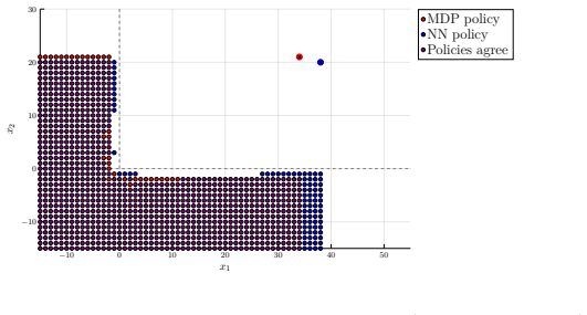
In low dimensions the method captures the geometry of the optimal policy, not just its cost: the learned ordering boundary overlaps the MDP solution in the reported 2-D figures, suggesting the value-function representation carries enough information to recover the (sigma,S) structure.
The continuous-time impulse-control approximation is close enough to the discrete-time problem that policies derived from it are directly usable: all performance comparisons are run in the original discrete-time formulation, and the gap to optimality stays small.
The same training pipeline — penalty-augmented inequality loss plus reference-process exploration — should apply to other impulse-control and fixed-cost control problems, such as cash management or optimal switching, where the value function satisfies the same kind of stochastic-target identity.

Reading between the lines

Editorial extensions of the paper, not claims the author makes directly.

The paper does not test, but it follows from the design that the method currently borrows strength from the very heuristics it aims to beat: the reference process is centered on the order-up-to vector of a tuned benchmark. A natural test is to run training with a crude or self-tuned reference policy and see whether the neural network still solves the problem, which would show whether the method is
The paper does not quantify, but a formal bound on the gap between the discrete-time MDP value and the continuous-time impulse-control value would turn the empirical near-optimality into a guarantee; the reported success with Poisson and negative binomial demands suggests the approximation error is small, but the assumption is only tested indirectly.
The deployment bottleneck is policy extraction: simulating one trace takes 1-4 hours because of Hessian evaluation and numerical minimization, while the alternative gradient-stationarity condition G(z*) = -c is much cheaper; systematic use of the latter could make the method practical for routine weekly reviews.
The clearest edge over heuristics appears when demand variability is moderate to high and backlog penalties are large; a targeted comparison on high-dimensional problems with correlated or heavy-tailed demand would test whether that edge persists outside the tested distributions.

Share X Bluesky LinkedIn Reddit HN

Editorial analysis

A structured set of objections, weighed in public.

Desk editor's note, referee report, and a circularity audit.

Desk Editor's Note

read the letter

What you should know: this is the first computationally feasible attempt at the high-dimensional stochastic joint replenishment problem with fixed costs, and the low-dimensional validation is genuinely strong. The authors extend deep BSDE methods to impulse control by dualizing an almost-sure inequality into a penalty loss and by designing reference processes with state-dependent jumps. That is real novelty, and they back it with code and careful benchmarks.

The theoretical soft spot is exactly where the stress-test puts it. Eq. (15) is the foundation of the loss, and the formal derivation in Appendix A reduces it to Lemma 1. Condition (i) follows from the HJB. Condition (ii) does not: the change-of-measure argument is asserted, not supplied, and the cited papers do not cover this specific randomized Poisson/lognormal reference process. The authors themselves say they are not attempting rigorous justification. If (ii) fails, the loss is minimized at something below the true value function and the extracted policy loses its theoretical grounding. This is load-bearing for the general claim—not for the empirical results, which could still hold—but it means the method's reliability in 12D and 50D rests on an unproved identity.

That said, the empirical work is credible. The 1D comparison to Sulem's exact solution and the 2D results within 1% of MDP are strong evidence that the identity works for at least those reference processes. The 12D and 50D results against tuned heuristics are extensive. I am less bothered than the stress-test by the benchmark-S entering only as the mean of the exploration distribution; that is an informed prior, not circularity. The bigger practical concerns are the 10 sample paths for 50D (small even if standard errors look fine) and per-problem hyperparameter tuning without a clean separation between tuning and evaluation. These are fixable with more paths and a validation protocol.

This paper deserves a serious referee. The theoretical gap should be addressed head-on—either a proof of condition (ii) for the reference class or a clear statement that the method is heuristic with strong empirical support. An editor should not desk-reject it; the contribution is significant and the authors are honest about the limits.

For a reading group, I'd bring it up if you work on deep BSDE methods or stochastic inventory. I would cite it as a method for high-dimensional impulse control, with a caveat on the theoretical gap.

Referee Report

2 major / 5 minor

Summary. The paper studies a discrete-time stochastic joint replenishment problem (SJRP) with fixed ordering costs and linear holding/backlog costs. It approximates this problem by a continuous-time impulse control problem, derives a probabilistic representation ('stochastic identity', Eq. (15)) connecting the value function to a stochastic target problem, and uses this identity to construct a deep-BSDE-style loss (Eq. (17)) trained on a randomized order-up-to reference process. A neural-network policy is extracted from the trained value/gradient networks via the HJB conditions (Eqs. (19)--(22)). The method is validated in one dimension against Sulem (1986), in two dimensions against an MDP policy iteration solution (within ~1% in seven test problems, Table 6), and in 12 and 50 dimensions against standard heuristics ((R,S), (Q,S), can-order, independent (s,S)). The authors claim the NN policy matches or beats the best benchmark in 36 high-dimensional test problems and is computationally feasible up to 50 SKUs. The paper provides code and details on hyperparameters and benchmark implementations.

Significance. If the main claims hold, this is a meaningful advance: it is one of the first methods to address the SJRP in 50 dimensions with fixed costs, a regime where exact MDP methods are intractable. The low-dimensional empirical validation is a genuine strength: the 2D comparisons against policy iteration (Table 6) and the 1D comparison against Sulem's analytical solution (Figure 3) provide concrete evidence that the algorithm can recover near-optimal policies in small problems. The paper also ships reproducible code, reports standard errors, and is careful in describing benchmark implementation. The key weakness is that the theoretical foundation — the stochastic identity (15) — is explicitly not rigorously proven for the reference process used, and the high-dimensional claims contain an internal inconsistency in the 'beats' terminology. These issues are load-bearing for the general claim of solving high-dimensional SJRPs, though the empirical contribution remains valuable.

major comments (2)

[§4 and Appendix A, Eq. (15), Lemma 1] The stochastic identity (15) is the theoretical basis of the loss (17), yet Appendix A does not establish condition (ii) of Lemma 1. The text says one 'can construct a sequence of processes' using a change-of-measure argument and cites Bouchard (2009) and Kharroubi et al. (2010), but those papers do not cover the specific randomized Poisson/lognormal reference process with state-dependent max jumps used here. If condition (ii) fails, the supremum in (15) is strictly below V(x), so minimizing (17) may not recover V, and the policy extraction (21)--(22) has no theoretical justification. The 1D and 2D experiments validate the method on particular test problems but do not establish the identity for the reference-process class used in 12D and 50D. Please either supply a rigorous proof of condition (ii) for this reference process, or explicitly state that (15) is a heuristic conjecture and qua
[§7, 'Results in dimension 50' and Table 7] The text states: 'The NN policy beats the best benchmark in all cases' for the 50-dimensional problems. This is contradicted by Table 7: for the three Poisson rows, the best benchmark is (Q,S) with gaps of 0.64%, 0.58%, and 0.59%, all below the paper's own 1% threshold for 'beats'. These cases should be labeled as 'matches', not 'beats'. Additionally, the NN performance in Table 7 is estimated from only 10 simulated sample paths per problem. Even if the reported standard errors are small, 10 independent replications is a thin basis for the central high-dimensional claim, especially for gaps near the 1% threshold. Please correct the terminology and either provide more replications or report confidence intervals that account for the small number of paths.

minor comments (5)

[Algorithm 1, line 8] The line uses ζ_j in the max{·,·} expression, but the generated vectors are denoted ζ_n. Also, the max operation is said to be applied componentwise, but the operands are not clearly aligned; please clarify the notation (e.g., define the componentwise max explicitly).
[§4, Eq. (16)] Setting E[Z_j] to the benchmark S means the reference process is centered at the benchmark's order-up-to vector. This is reasonable as an exploration device, but it should be discussed as a possible source of favorable bias when the paper later claims to match or beat those same benchmarks. An ablation with a different center (e.g., a fixed heuristic) would strengthen the claim.
[§7, Tables 3--5] The tables report negative gaps (benchmark cost lower than NN cost) as well as positive gaps, but the caption does not explain the sign convention. A reader may not immediately see that a negative entry means the benchmark performs slightly better; please state this explicitly.
[Appendix B.2, hyperparameter tables] Several tuning parameters (T, λ, ν, α, β_final, ε, box bounds) are listed per test problem, but the process for choosing them is described only qualitatively. Reporting the search ranges or the number of tuning runs would improve replicability.
[Abstract and §1] The phrase 'solves the SJRP in high dimensions' overstates the contribution given the lack of a rigorous proof of the identity (15). The empirical results are strong, but the wording should be tempered to 'computes an effective policy' or 'matches or beats benchmarks'.

Circularity Check

0 steps flagged · score 1.0 of 10

No load-bearing circularity: the central identity is derived from HJB and Itô, not from benchmarks; the benchmark S enters only as an exploration prior. The unproved condition (ii) in Appendix A is a correctness gap, not a circular step.

full rationale

The paper's claimed derivation chain is not circular. The core theoretical input is the stochastic identity (15), which is formally derived in Appendix A from the HJB equation (12) via Itô's formula, not assumed from the benchmark policies. Lemma 1 reduces (15) to two conditions: (i) A+B≤0 a.s., which follows directly from the HJB equation, and (ii) P(A+B>−w)>0 for all w>0, which is asserted via a change-of-measure argument with citations to Bouchard (2009) and Kharroubi et al. (2010) — external works, not self-citations. If (ii) were false, the loss (17) would not recover V, but that would be an invalidity gap, not circularity, since the identity is not assumed from the conclusion. The benchmark policies (R,S), (Q,S), can-order, and independent (s,S) are evaluated externally in the original discrete-time model, and the NN policy is obtained from the learned value/gradient approximations via (21)-(22). The only benchmark information entering training is E[Z]=S (Eq. 16), used as the mean of the exploration distribution, and in the 2-D tests a nearby MDP-derived E[Z] with optimization bounds scaled by it. This is a warm-start/exploration prior, not the final policy formula, and the reported performance is obtained by simulating the extracted policy, so no equality is forced by construction. There is no self-citation chain bearing the central claim, no imported uniqueness theorem, and no renaming of a known result. The unproved stochastic identity and the benchmark-informed exploration mean are genuine limitations to verify, but they do not make the derivation circular.

Assumptions & free parameters 7 free parameters · 5 assumptions · 0 invented entities

The method relies on no new physical or mathematical entities. The free parameters are algorithm hyperparameters chosen per test problem. The main axioms are the validity of the stochastic identity (not rigorously proved in the paper) and the Brownian approximation of the original demand model. These are domain assumptions rather than standard mathematical facts, and they are load-bearing for the method.

free parameters (7)

reference order rate λ = Varies per problem (e.g., 4.00, 1.73, 0.4)
Sets the frequency of jumps in the reference process; chosen per test problem to balance exploration and stability.
exploration variance ν = Varies per problem (e.g., 0.2, 0.4, 0.8)
Scales the variance of the lognormal order-up-to sampling distribution Φ; controls the degree of state-space exploration.
exponential mean scale α = Varies per problem (e.g., 0, 0.2, 0.4)
Determines the mean of the exponential exploration noise ζ (mean α_i = α μ_i / λ); must satisfy α<1 for reference process stability.
time horizon T = Varies per problem (e.g., 0.1, 0.05, 0.2)
Training horizon in the loss function; tuned empirically for each problem.
final penalty β_final = Varies per problem (e.g., 10^5, 10^6, 10^7)
Controls the weight of the stochastic-inequality violation penalty in the loss; tuned per problem to keep violation probability below 1%.
cost scaling κ = 0.1 or 0.01
Scales all costs for numerical stability; does not affect the optimal policy (Appendix B.1).
exploration center E[Z] = S vector of (Q,S) or can-order benchmark
Sets the mean of the lognormal order-up-to sampling distribution to a benchmark's order-up-to level; used to guide exploration toward relevant regions.

assumptions (5)

domain assumption The stochastic identity (Eq. 15) is valid for the impulse control problem and the chosen reference process
The paper provides only a formal derivation (Appendix A) and cites Bouchard (2009) and Kharroubi et al. (2010) for rigorous treatments; the identity is the foundation of the loss function (Eq. 17).
domain assumption The continuous-time Brownian demand D(t)=μt+σB(t) approximates the original discrete-time demand process well enough for policy transfer
The original problem is discrete-time with Poisson or negative binomial demand; the method solves a Brownian approximation (Eq. 8) and transfers the policy back to the discrete-time problem.
standard math The value function V is sufficiently smooth (C^2) for Itô's lemma and the HJB equation
Needed for the formal derivation in Eq. (26) and for classical solutions of the HJB equation (12).
domain assumption There exists an optimal (σ,S)-type policy, and the order-up-to vector z* is independent of the state for x ≤ z*
Used to justify extracting a single order-up-to level from the NN (Eq. 24); follows from Johnson (1967) for the discrete-time problem, as discussed in Section 4.
domain assumption The reference process is stable under the condition λ E[ζ] < μ_i (i.e., α<1)
Stated in Section 4 to ensure the reference process does not drift to -∞; required for meaningful simulation.

how reviews work

0 comments

Cite this review

Pith. "Pith review of A Computational Method for Solving the Stochastic Joint Replenishment Problem in High Dimensions." pith.science (2026). https://pith.science/paper/BSAYWCI4

@misc{pith2026251111830,
  author       = {Pith},
  title        = {Pith review of: A Computational Method for Solving the Stochastic Joint Replenishment Problem in High Dimensions},
  year         = {2026},
  howpublished = {\url{https://pith.science/paper/BSAYWCI4}},
  note         = {Machine review of arXiv:2511.11830}
}

read the original abstract

We consider a discrete-time formulation for a class of high-dimensional stochastic joint replenishment problems. First, we approximate the problem by a continuous-time impulse control problem. Exploiting connections among the impulse control problem, backward stochastic differential equations (BSDEs) with jumps, and the stochastic target problem, we develop a novel, simulation-based computational method that relies on deep neural networks to solve the impulse control problem. Based on that solution, we propose an implementable inventory control policy for the original (discrete-time) stochastic joint replenishment problem, and test it against the best available benchmarks in a series of test problems. For the problems studied thus far, our method matches or beats the best benchmark we could find, and it is computationally feasible up to at least 50 dimensions -- that is, 50 stock-keeping units (SKUs).

Figures

Figures reproduced from arXiv: 2511.11830 by the authors.

**Figure 1.** MDP and neural network policies (base case d = 2). −10 0 10 20 30 40 50 −10 0 10 20 30 x1 x2 (a) Low CV −10 0 10 20 30 40 50 −10 0 10 20 30 x1 x2 (b) High CV −10 0 10 20 30 40 50 −10 0 10 20 30 x1 x2 (c) p = 10 −10 0 10 20 30 40 50 −10 0 10 20 30 x1 x2 (d) p = 100 −10 0 10 20 30 40 50 −10 0 10 20 30 x1 x2 (e) c0 = 20 −10 0 10 20 30 40 50 −10 0 10 20 30 x1 x2 (f) c0 = 100 [PITH_FULL_IMAGE:figures/full_fig_p028_1.png] view at source ↗

**Figure 2.** Comparison of MDP and neural network policies across the remaining six twodimensional test problems. 28 [PITH_FULL_IMAGE:figures/full_fig_p028_2.png] view at source ↗

**Figure 3.** Value function and gradient computed using the expressions in Sulem (1986), and the neural network approximations 52 [PITH_FULL_IMAGE:figures/full_fig_p052_3.png] view at source ↗

Discussion (0). Continue with ORCID to comment.

Forward citations

Cited by 1 Pith paper

Reviewed papers in the Pith corpus that reference this work. Sorted by Pith novelty score. Full citation record

Deep Learning Method for Stationary Distribution of Reflected Brownian Motion
cs.LG 2026-07 conditional novelty 6.5 of 10

A carefully regularized neural network trained on the BAR residual recovers Laplace transforms of high-dimensional RBM stationary distributions well enough for near-exact tail-probability inversion up to 30 dimensions.

Reference graph

Works this paper leans on

12 extracted references · 1 linked inside Pith · cited by 1 Pith paper

[1]

can-order

Adelman, D. and Klabjan, D. (2005). Duality and existence of optimal policies in generalized joint replen- ishment.Mathematics of Operations Research, 30(1):28–50. Adelman, D. and Klabjan, D. (2012). Computing near-optimal policies in generalized joint replenishment. INFORMS Journal on Computing, 24(1):148–164. Aksoy, Y. and Erenguc, S. (1988). Multi-item...

2005
[4]

Also recall the corresponding reference process ˜X(·) given by (14): ˜X(t) =x−µt−σB(t) + X j:Tj ≤t Yj. Formally applying a generalized Itˆ o’s lemma for jump diffusion to the function (x, t)7→e −rtV(x) (see, e.g., Applebaum (2009)), we have e−rT V( ˜X(T))−V(x) = Z T 0 e−rt −rV−LV ( ˜X(t−))dt− Z T 0 e−rt∇V( ˜X(t−)) ⊤σ dB(t) + X j:Tj ≤T e−rTj h V( ˜X(T j))−...

2009
[5]

Can-order policy .A can-order policy is specified by 3dparameters, reorder pointss i, can- order pointso i, and order-up-to levelsS i,i= 1,

P E[Di]⌋}in order to find the optimalQ ∗. Can-order policy .A can-order policy is specified by 3dparameters, reorder pointss i, can- order pointso i, and order-up-to levelsS i,i= 1, . . . , d, withsi ≤o i ≤S i for eachi. Whenever the inventory level of some item, say itemi, drops to or belows i, an order is placed. For itemi, the order raises its inventor...

1986
[7]

Given thatA(X ∗) = 0 andB(X ∗) = 0 a.s., we wish to show thatP(A( ˜X) +B( ˜X)>−w)>0 for anyw >0

Thus, the no-action term in (12) is zero for allt >0, a.s., implying thatA(X ∗) = 0 a.s. Given thatA(X ∗) = 0 andB(X ∗) = 0 a.s., we wish to show thatP(A( ˜X) +B( ˜X)>−w)>0 for anyw >0. To achieve this, one can construct a sequence of processes, starting with the reference process ˜X, that increasingly favors the optimal state trajectories, using a change...

2009
[10]

Whenα= 1, we call the corresponding policy the vanilla independent (s, S) policy

In other words, the independent (s, S) policies differ only in the fixed cost used to determine thes i andS i levels. Whenα= 1, we call the corresponding policy the vanilla independent (s, S) policy. The vanilla policy is a common and natural benchmark used in the literature (see, e.g., Atkins and Iyogun, 1988; Viswanathan, 1997). We consider a larger fam...

1988
[29]

Veinott Jr, A

Springer Science & Business Media. Veinott Jr, A. F. and Wagner, H. M. (1965). Computing optimal (s, S) inventory policies.Management Science, 11(5):525–552. Viswanathan, S. (1996). A new optimal algorithm for the joint replenishment problem.Journal of the Operational Research Society, 47(7):936–944. Viswanathan, S. (1997). Note. Periodic review (s, S) po...

1965
[43]

Zheng, Y.-S

Springer Science & Business Media. Zheng, Y.-S. and Federgruen, A. (1991). Finding optimal (s, S) policies is about as simple as evaluating a single policy.Operations Research, 39(4):654–665. 34 A. Formal Derivation of Stochastic Identity(15) Recall the value functionVdefined in Eq. (11).Vis a formal solution to the HJB equation (12). LetT >0, and letU(·;...

1991
[153]

Pham, H., Warin, X., and Germain, M. (2021). Neural networks-based backward scheme for fully nonlinear PDEs.SN Partial Differential Equations and Applications, 2(1):16. Porteus, E. L. (1971). On the optimality of generalized (s, S) policies.Management Science, 17(7):411–426. Roundy, R. (1985). 98%-effective integer-ratio lot-sizing for one-warehouse multi...

2021

Show all 12 references

[297]

A simple method of determining order quantities in joint replen- ishments under deterministic demand

30 Bayraktar, E., Cohen, A., and Nellis, A. (2023). A neural network approach to high-dimensional opti- mal switching problems with jumps in energy markets.SIAM Journal on Financial Mathematics, 14(4):1028–1061. Beck, C., Hutzenthaler, M., Jentzen, A., and Kuckuck, B. (2022). ...

2023 arXiv
[1250]

During training, we use learning rates 10 −3, 10−4, and 10−5 consecutively, each for 5000 iterations, to achieve high accuracy

For the neural-network architecture, the hidden layers have width 250, and we use four hidden layers with ELU activation functions in this one-dimensional example. During training, we use learning rates 10 −3, 10−4, and 10−5 consecutively, each for 5000 iterations, to achieve ...

1986
[2006]

inOptim.jl. Since the neural network approximations are reliable only in regions of the state space that were sufficiently explored during training, we impose box constraints to confine the search forz ∗ to a domain we expect has been learned well. We implement these constrain...

2023
[2018]

in theJulia 1.10computing language (Bezanson et al., 2017). Currently, we conduct the numerical experiments on a high-performance computing node equipped with an NVIDIA H100 GPU with 80 GB memory and an AMD EPYC 9334 32-core processor, allowing up to 64 logical threads, with 6...

2017

Pith tools

Reviewed August 3, 2026 · model on record in the stance chip above.

[1] [1]

can-order

Adelman, D. and Klabjan, D. (2005). Duality and existence of optimal policies in generalized joint replen- ishment.Mathematics of Operations Research, 30(1):28–50. Adelman, D. and Klabjan, D. (2012). Computing near-optimal policies in generalized joint replenishment. INFORMS Journal on Computing, 24(1):148–164. Aksoy, Y. and Erenguc, S. (1988). Multi-item...

2005

[2] [4]

Also recall the corresponding reference process ˜X(·) given by (14): ˜X(t) =x−µt−σB(t) + X j:Tj ≤t Yj. Formally applying a generalized Itˆ o’s lemma for jump diffusion to the function (x, t)7→e −rtV(x) (see, e.g., Applebaum (2009)), we have e−rT V( ˜X(T))−V(x) = Z T 0 e−rt −rV−LV ( ˜X(t−))dt− Z T 0 e−rt∇V( ˜X(t−)) ⊤σ dB(t) + X j:Tj ≤T e−rTj h V( ˜X(T j))−...

2009

[3] [5]

Can-order policy .A can-order policy is specified by 3dparameters, reorder pointss i, can- order pointso i, and order-up-to levelsS i,i= 1,

P E[Di]⌋}in order to find the optimalQ ∗. Can-order policy .A can-order policy is specified by 3dparameters, reorder pointss i, can- order pointso i, and order-up-to levelsS i,i= 1, . . . , d, withsi ≤o i ≤S i for eachi. Whenever the inventory level of some item, say itemi, drops to or belows i, an order is placed. For itemi, the order raises its inventor...

1986

[4] [7]

Given thatA(X ∗) = 0 andB(X ∗) = 0 a.s., we wish to show thatP(A( ˜X) +B( ˜X)>−w)>0 for anyw >0

Thus, the no-action term in (12) is zero for allt >0, a.s., implying thatA(X ∗) = 0 a.s. Given thatA(X ∗) = 0 andB(X ∗) = 0 a.s., we wish to show thatP(A( ˜X) +B( ˜X)>−w)>0 for anyw >0. To achieve this, one can construct a sequence of processes, starting with the reference process ˜X, that increasingly favors the optimal state trajectories, using a change...

2009

[5] [10]

Whenα= 1, we call the corresponding policy the vanilla independent (s, S) policy

In other words, the independent (s, S) policies differ only in the fixed cost used to determine thes i andS i levels. Whenα= 1, we call the corresponding policy the vanilla independent (s, S) policy. The vanilla policy is a common and natural benchmark used in the literature (see, e.g., Atkins and Iyogun, 1988; Viswanathan, 1997). We consider a larger fam...

1988

[6] [29]

Veinott Jr, A

Springer Science & Business Media. Veinott Jr, A. F. and Wagner, H. M. (1965). Computing optimal (s, S) inventory policies.Management Science, 11(5):525–552. Viswanathan, S. (1996). A new optimal algorithm for the joint replenishment problem.Journal of the Operational Research Society, 47(7):936–944. Viswanathan, S. (1997). Note. Periodic review (s, S) po...

1965

[7] [43]

Zheng, Y.-S

Springer Science & Business Media. Zheng, Y.-S. and Federgruen, A. (1991). Finding optimal (s, S) policies is about as simple as evaluating a single policy.Operations Research, 39(4):654–665. 34 A. Formal Derivation of Stochastic Identity(15) Recall the value functionVdefined in Eq. (11).Vis a formal solution to the HJB equation (12). LetT >0, and letU(·;...

1991

[8] [153]

Pham, H., Warin, X., and Germain, M. (2021). Neural networks-based backward scheme for fully nonlinear PDEs.SN Partial Differential Equations and Applications, 2(1):16. Porteus, E. L. (1971). On the optimality of generalized (s, S) policies.Management Science, 17(7):411–426. Roundy, R. (1985). 98%-effective integer-ratio lot-sizing for one-warehouse multi...

2021