KAN vs LSTM Performance in Time Series Forecasting

Federico Frascoli; Nadezda Sukhorukova; S M Mahmudul Hasan Joy; Tabish Ali Rather

REVIEW 4 major objections 5 minor 38 references

KAN vs LSTM Performance in Time Series Forecasting

T0 review · 4 major / 5 minor · reviewed 2026-08-03 · deepseek-v4-flash

Challenge this review Re-run · record.json Download PDF Read on arXiv ↗ Review JSON

Pith's one-line read LSTM beats baseline KAN by 6.5–10x on stock-price forecasts, the paper shows.

desk verdict The 7-10x LSTM advantage in Table 3 is not backed by the paper's own numbers; the qualitative claim is plausible but the magnitudes are unverified. read the letter →

arxiv 2511.18613 v2 pith:FTEMZB6E submitted 2025-11-23 cs.LG cs.AI

Tabish Ali Rather , S M Mahmudul Hasan Joy , Nadezda Sukhorukova , Federico Frascoli This is my paper · ORCID

classification cs.LGcs.AI MSC 68T0762M1091G80

keywords timeseriesforecastingLSTMKolmogorov-ArnoldNetworksstockpricepredictionRMSEinterpretabilityforecasthorizondeeplearning

verification ladder T0 review T1 audit T2 compute T3 formal

The pith

A machine-rendered reading of the paper's core claim, the machinery that carries it, and where it could break.

The reading

This paper tries to establish a performance baseline between two neural architectures on stochastic financial time series: Long Short-Term Memory networks and standard Kolmogorov-Arnold Networks. Using a direct multi-output forecasting protocol with 20-day look-back windows and RMSE in normalized space, the authors report that LSTM achieves 6.5 to 10 times lower error than KAN across 1-day, 2-day, and 100-day horizons and three market conditions. They also find KAN trains about 2.1 times faster and offers theoretical interpretability through the Kolmogorov-Arnold representation theorem, but this does not offset its accuracy gap. The claim matters because it informs architecture selection for accuracy-critical forecasting and motivates specialized temporal KAN variants rather than standard KAN.

What carries the argument

The comparison is carried by the two architectures themselves: LSTM, a gated recurrent network that mitigates vanishing gradients and captures long-term dependencies, and KAN, which replaces fixed node activations with learnable univariate spline functions grounded in the Kolmogorov-Arnold representation theorem, where a multivariate function decomposes into sums of univariate functions. The theorem supplies KAN's interpretability rationale but does not model temporal dependencies, which the paper identifies as the root of KAN's sequential-data weakness. The evaluation machinery is a direct multi-output forecasting protocol: 20-day look-back windows, iterative single-step prediction, and RMS

What would settle it

Retrain both architectures on the same dataset with hyperparameters chosen on a held-out validation set, average over at least five random seeds, and report test RMSE with confidence intervals. If LSTM's advantage over KAN falls below about 2x or is not statistically significant, the claimed 6.5–10x superiority is an artifact of test-set selection.

Watch

Extended reading notes

Core claim

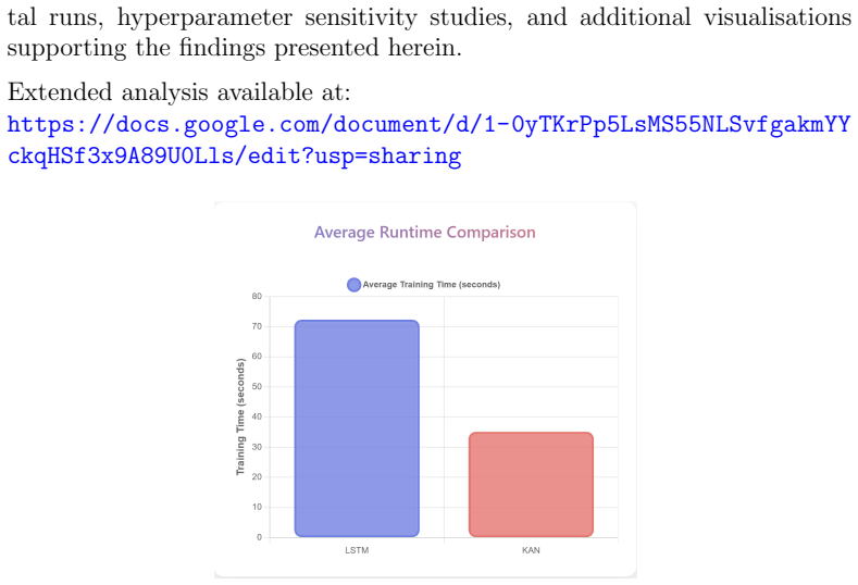
The central discovery, on the paper's own terms, is that baseline KAN, implemented in its standard form, is not competitive with LSTM for stock price forecasting. On normalized RMSE, LSTM's best configurations achieve 0.039 (1-day normal market) versus KAN's 0.390, a 10-fold advantage; across all horizons and market types the advantage stays between 6.5 and 10 times. KAN's training-time advantage (averaging 35.12 seconds vs about 75 seconds) and interpretability are confirmed, and KAN can produce forecasts at 200-day horizons where the paper reports no LSTM result, but the accuracy gap dominates. The authors conclude that LSTM should be the default for practical financial forecasting, while

Load-bearing premise

The comparison's validity depends on the premise that the per-horizon 'Best Config' values in Table 3 are fair representations of each architecture, rather than artifacts of test-set-based model selection.

Editorial extensions

If this is right

For accuracy-critical financial forecasting, LSTM remains the evidence-supported default until specialized KAN variants change the picture.
Standard KAN may still fit rapid prototyping and resource-constrained deployments, where its ~2x faster training matters more than accuracy.
The results bound the value of theoretical interpretability: transparency alone does not make an architecture practically useful for sequential prediction.
The gap motivates mathematical research into free-knot polynomial spline approximation, since KAN's optimization difficulty is cited as the main blocker.
Specialized temporal KAN variants (e.g., Time-Frequency KAN) are outside this study's scope but are the natural next targets for evaluation.

Reading between the lines

Editorial extensions of the paper, not claims the author makes directly.

The reported 6.5–10x advantage may be inflated because the best configuration per horizon was selected directly on the test set, without a validation set or repeated-seed averaging; a fairer protocol could shrink the gap.
The paper's phrasing that KAN can forecast 200 days where LSTM fails likely reflects that LSTM was not trained at that horizon rather than an inherent limitation; a head-to-head at 200 days would settle it.
Since KAN uses a different optimizer (LBFGS) and smaller parameter budgets in the reported runs, its '2.1x faster training' may partly reflect optimizer and capacity differences, not a fundamental architectural advantage.
If the accuracy gap is real, then for non-stationary financial series, KAN's spline activations may be too rigid to track regime changes; a testable extension is to feed KAN with differenced or volatility-adjusted inputs.

Share X Bluesky LinkedIn Reddit HN

Signed reviews

No signed human review yet.

Editorial analysis

A structured set of objections, weighed in public.

Desk editor's note, referee report, and a circularity audit.

Desk Editor's Note

read the letter

Here's my take. The paper's central result—LSTM beats vanilla KAN by 6.5-10x in RMSE—does not hold up against the paper's own tables. Table 1 shows the best LSTM test RMSE at 0.0745; Table 3 reports 0.039 for the same 1-day normal market. Table 2 shows the best KAN test RMSE at 0.152; Table 3 reports 0.390. The 10x ratio comes from numbers that appear nowhere in the experimental record. There are also duplicated rows in Table 2 (configs 1/2 and 5/6 have identical train/test RMSE despite different hyperparameters), and the 200-day LSTM rows are N/A while the abstract claims superiority 'across all tested prediction horizons' and the discussion says LSTM faces computational constraints—without showing any experiment.

To be fair, the paper does some things well. It is explicit that the comparison is only between baseline architectures, and it correctly notes that specialized KAN variants are out of scope. The qualitative direction—LSTM outperforms standard KAN on sequential data—is consistent with prior work the authors cite, so the conclusion isn't surprising. The 2.1x training speed advantage for KAN is a modest practical point, though it's based on runtime averages without much detail.

The soft spots are load-bearing. No error bars or seed averaging; the 'best config' per horizon is selected using test RMSE, so the reported advantage is partly a test-set fit. The dataset is not described (which stock? what period? how many points?), and the code URL contains a space and is presumably broken. The paper itself concedes in the introduction that standard KAN has shown limited effectiveness for sequential data, citing a critique, so the main finding is not new.

Given these problems, the paper is a small empirical replication with unreliable numbers. It could become a useful baseline if the authors fix the tables, add validation-based selection and variance reporting, and describe the data. As it stands, I wouldn't cite it, and I wouldn't send it to a serious referee—the internal contradictions would waste everyone's time. For a reading group, it's a decent case study in how benchmark comparisons can go wrong, but not for its positive results.

Referee Report

4 major / 5 minor

Summary. The paper reports a controlled empirical comparison of baseline Kolmogorov-Arnold Networks (KAN, implemented with PyKAN) and Long Short-Term Memory (LSTM) networks for forecasting stock price data. Accuracy is measured by RMSE in normalized feature space under a direct multi-step forecasting protocol with 20-day look-back windows. The central claim is that LSTM achieves 6.5–10x lower RMSE across 1-day, 2-day, 100-day, and (where available) 200-day horizons, while KAN trains about 2.1x faster. The paper further argues for complementary roles: LSTM for accuracy-critical short-term forecasting and KAN for interpretability, speed, and extended-horizon forecasts. The scope is explicitly limited to baseline KAN and baseline LSTM, excluding specialized temporal KAN variants.

Significance. If the quantitative claims were reliable, the paper would provide a useful benchmark for baseline KAN on stochastic financial time series and would reinforce the established view that LSTM remains the default for accuracy-critical sequential forecasting. Strengths include the direct architecture-to-architecture comparison, open code links, and an explicit scope limitation to baseline variants. However, the current manuscript's central magnitude claim is not verifiable from its own tables: the LSTM/KAN RMSEs in Table 3 do not match the model-selection tables, and the configuration selection protocol is invalid for generalization claims. These issues make the headline 7–10x advantage unsupported as presented.

major comments (4)

[§5.4, Table 3 vs Tables 1 and 2] The central RMSE values underlying the 6.5–10x advantage are not present in the experiments reported earlier. Table 3 lists LSTM 1-day RMSE as 0.039 with '100u-linear' as best config, but Table 1 reports this exact configuration (4 layers, 100 units, linear) with test RMSE 0.0829 and reports the overall best LSTM test RMSE as 0.0745 (2 layers, 10 units, tanh). Similarly, Table 3 lists KAN 1-day RMSE as 0.390, while Table 2 reports all KAN test RMSEs in the range 0.152–0.331. The paper must reconcile these numbers or state the exact data split, normalization, and evaluation protocol that produced Table 3; otherwise the headline accuracy advantage is unsupported by the paper's own evidence.
[§5.4 and §4.1–4.2] The 'Best Config' column in Table 3 is selected from test RMSE values, with no validation set, no seed averaging, and no confidence intervals. For example, the 1-day LSTM config is '100u-linear' despite Table 1 showing this config with higher test RMSE than the 10u-tanh config; the selection appears to be an a posteriori choice based on the test set. This makes the reported 7–10x advantage an upper-bound artifact of test-set fitting rather than a fair architectural comparison. A proper protocol should use a validation split for model selection and report mean and variance over multiple random initializations or, at minimum, a clear statement of how configurations were chosen without access to test labels.
[§5.4, §5.5, §5.6, and Abstract] There is an internal contradiction about the 200-day horizon. Table 3 reports LSTM RMSE as N/A for all 200-day rows, while the abstract and §5.4 claim LSTM is superior 'across all tested prediction horizons,' and §5.5 lists LSTM as 'best overall' without excluding 200-day. The discussion also states that LSTM 'faces computational constraints beyond 100-day predictions' (§5.6), but no runtime or memory evidence for this claim is provided. Either include LSTM results for the 200-day horizon or explicitly restrict all superiority claims to horizons where LSTM was actually run.
[§5.2, Table 2; §3.2] Table 2 contains duplicate rows: Config 1 (grid=3, k=6) and Config 2 (grid=3, k=2) have identical train/test RMSE (0.274/0.188), and Configs 5 and 6 (differing only in number of neurons) also have identical RMSEs (0.274/0.152). This suggests misreported or insufficiently described experiments. Additionally, the manuscript does not specify the stock, the time period, the train/test split size, or how the 'Normal/Volatile/Trending' market conditions are defined and labeled. These details are essential to reproduce or interpret any of the tables.

minor comments (5)

[§1 and §5.6] The term 'non-deterministic' is used loosely for stochastic financial data; consider using 'stochastic' or 'noisy' consistently, since true non-determinism is a stronger mathematical claim.
[§5.3 and Figure 7] Runtime comparisons (35.12s vs ~75s) lack hardware details, number of runs, and standard deviations. The claim of '82.6% of training instances completing under 60 seconds' needs a denominator and a clear description of how it was measured.
[§7 Appendix] The GitHub repository name 'grand challenges 2024' and the Google Docs supplementary link are not stable or archival; the code and additional results should be deposited in a permanent repository (e.g., Zenodo) with a version/DOI.
[Tables 1 and 3] Minor typographical issues: 'T rain RMSE' in Table 1, and 'KANs Only' in Table 3's Best Config column. Also, Table 3 does not define '100u-linear' vs '10u-tanh-100'—these abbreviations should be explained in the caption or text.
[General] Some references are listed twice ([14] and [15] are the same paper) and some are not consistently formatted. A careful proofreading pass is needed.

Circularity Check

0 steps flagged · score 0.0 of 10

No circular derivation; the paper is a direct empirical comparison with no reduction of its claims to its inputs.

full rationale

The paper contains no derivation chain whose output is equivalent to its input by construction. Its central claim—LSTM RMSE 0.039 vs KAN RMSE 0.390 and a 6.5–10x advantage—is presented as the measured outcome of training and test experiments in Tables 1–3, not as a quantity defined in terms of the models or fitted from the same data. The Kolmogorov-Arnold theorem is imported as standard external mathematics ([19], [23]) and is not used to force the empirical performance comparison. Manual hyperparameter tuning and selection of the 'Best Config' from test results is a model-selection/generalization concern, not a circularity of the kind where a fitted parameter is renamed as a prediction. The internal inconsistencies noted by the skeptic, such as Table 3 values not matching Tables 1–2 and the 200-day rows lacking LSTM values, are reproducibility and consistency problems rather than definitional or self-citation circularity. No load-bearing self-citation appears: the author-related references ([34], [36]) provide background on spline optimization and do not establish the comparative outcome. Therefore no specific circular step can be exhibited, and the appropriate score is 0.

Assumptions & free parameters 5 free parameters · 4 assumptions · 0 invented entities

The central claim rests on hand-tuned hyperparameters—several selected using test-set RMSE—and on unverified domain assumptions about the dataset and PyKAN implementation. No derivation provides independent support for these choices.

free parameters (5)

LSTM best configuration (1-day) = 4 layers, 100 units, linear activation
Selected as best based on test RMSE in Table 3; effectively fit to the test set for that horizon.
LSTM best configuration (2-day and 100-day) = 2 layers, 10 units, tanh (2-day); 2 layers, 10 units, tanh, seq 100 (100-day)
Chosen per horizon from test RMSE values; no validation set is described, so these are hand-selected on test performance.
KAN hyperparameters = grid=3, k=2, neurons=len(train_input)//10
Manual tuning explained in §4.2; the optimal settings are identified using test RMSE.
Look-back window = 20 days
Fixed by hand; sensitivity not tested, yet all results depend on it.
Data scaling = Min-Max to [0,1]
Standard preprocessing, but the scaling constants are data-dependent and not reported.

assumptions (4)

standard math Kolmogorov-Arnold representation theorem (Eq. 1)
Used as theoretical grounding for KAN in §2.2.1; stated without proof, which is acceptable as a classical theorem.
domain assumption The yfinance data are correct and representative
The dataset is not described (no tickers, date range, or sample size); all experimental conclusions depend on this unspecified data source.
domain assumption PyKAN is a faithful implementation of standard KAN
Results are only for the PyKAN library as used here; the paper does not verify that the implementation matches the theoretical KAN architecture.
domain assumption RMSE on normalized prices is an appropriate comparison metric
The whole evaluation rests on RMSE; other metrics or trading-based evaluation could change relative rankings.

how reviews work

0 comments

Cite this review

Pith. "Pith review of KAN vs LSTM Performance in Time Series Forecasting." pith.science (2026). https://pith.science/paper/FTEMZB6E

@misc{pith2026251118613,
  author       = {Pith},
  title        = {Pith review of: KAN vs LSTM Performance in Time Series Forecasting},
  year         = {2026},
  howpublished = {\url{https://pith.science/paper/FTEMZB6E}},
  note         = {Machine review of arXiv:2511.18613}
}

read the original abstract

This study presents a controlled comparison of baseline Kolmogorov-Arnold Networks (KAN), implemented via PyKAN, and Long Short-Term Memory (LSTM) networks for the forecasting of stochastic, non-stationary financial time series. The two architectures are assessed in terms of predictive accuracy, computational efficiency, and interpretability, with accuracy measured by the Root Mean Square Error (RMSE) in normalised feature space. Under a direct multi-output forecasting protocol, LSTM attains clearly superior accuracy across all tested prediction horizons, consistent with its well-established effectiveness for sequential data modelling. Baseline KAN, although offering theoretical interpretability through the Kolmogorov-Arnold representation theorem, exhibits substantially higher error rates and limited practical applicability for time series forecasting in its standard form. Several specialised temporal variants -- including Temporal KAN and Time-Frequency KAN -- have since been proposed to address these sequential modelling limitations, but they lie outside the scope of the present study. KAN is observed to converge faster during training under the configurations tested, although direct runtime comparisons are constrained by methodological factors. These findings support the adoption of LSTM for accuracy-critical financial forecasting and establish an empirical baseline for standard KAN on stochastic sequential data, motivating further investigation of temporally-aware KAN architectures. The study benchmarks baseline KAN against baseline LSTM only; the results do not extend to specialised KAN variants designed for sequential data, nor to the broader family of temporal models.

Figures

Figures reproduced from arXiv: 2511.18613 by the authors.

**Figure 1.** LSTM representation [11] LSTM excel at retaining long-term dependencies while maintaining computational efficiency, establishing them as the preferred architecture for stock price prediction and other time series forecasting tasks [37, 35]. Their proven track record across diverse applications has made them the standard baseline for sequential modelling problems. 4 [PITH_FULL_IMAGE:figures/full_fig_p004_1.png] view at source ↗

**Figure 2.** Train and Test RMSE for Different LSTM Model Configurations [PITH_FULL_IMAGE:figures/full_fig_p009_2.png] view at source ↗

**Figure 3.** Train and Test Loss for Different KAN Configurations [PITH_FULL_IMAGE:figures/full_fig_p010_3.png] view at source ↗

Figures from the paper (5 more)

**Figure 4.** Figure 4: KAN vs LSTM Performance Comparison: 1-Day and 100-Day [PITH_FULL_IMAGE:figures/full_fig_p012_4.png]

**Figure 5.** Figure 5: KAN vs LSTM Performance Comparison: 2-Day and 200-Day [PITH_FULL_IMAGE:figures/full_fig_p012_5.png]

**Figure 6.** Figure 6: Time Series Forecasting: Actual vs LSTM vs KAN Predictions [PITH_FULL_IMAGE:figures/full_fig_p013_6.png]

**Figure 7.** Figure 7: Average Runtime Comparison: KAN vs LSTM Training Times. [PITH_FULL_IMAGE:figures/full_fig_p017_7.png]

**Figure 8.** Figure 8: KAN Architecture and Comparison with Traditional MLPs [ [PITH_FULL_IMAGE:figures/full_fig_p018_8.png]

Discussion (0). Continue with ORCID to comment.

Reference graph

Works this paper leans on

38 extracted references · 1 linked inside Pith

[1]

Mart ´ ın Abadi, Ashish Agarwal, Paul Barham, Eugene Brevdo, Zhifeng Chen, Craig Citro, Greg S. Corrado, Andy Davis, Jeffrey Dean, Matthieu Devin, Sanjay Ghemawat, Ian Goodfellow, Andrew Harp, Ge- offrey Irving, Michael Isard, Yangqing Jia, Rafal Jozefowicz, Lukasz Kaiser, Manjunath Kudlur, Josh Levenberg, Dandelion Man´ e, Ra- jat Monga, Sherry Moore, De...

2015
[2]

Springer, 18 Cham, 2nd edition, 2023

CC Aggarwal.Neural networks and deep learning: A textbook. Springer, 18 Cham, 2nd edition, 2023

2023
[3]

On functions of three variables.Doklady Akademii Nauk SSSR (Proceedings of the USSR Academy of Sciences), 114(4):679–681, 1957

VI Arnold. On functions of three variables.Doklady Akademii Nauk SSSR (Proceedings of the USSR Academy of Sciences), 114(4):679–681, 1957

1957
[4]

Github - ranaroussi/yfinance: Yahoo! finance market data downloader (+faster pandas datareader).https://github.com/ranar oussi/yfinance

Ran Aroussi. Github - ranaroussi/yfinance: Yahoo! finance market data downloader (+faster pandas datareader).https://github.com/ranar oussi/yfinance. Accessed: October 29, 2024

2024
[5]

Explainability and interpretability in electric load forecasting using machine learning techniques–a review.Energy and AI, page 100358, 2024

Lukas Baur, Konstantin Ditschuneit, Maximilian Schambach, Can Kaymakci, Thomas Wollmann, and Alexander Sauer. Explainability and interpretability in electric load forecasting using machine learning techniques–a review.Energy and AI, page 100358, 2024

2024
[6]

Mohit Beniwal, Archana Singh, and Nand Kumar. Forecasting multistep daily stock prices for long-term investment decisions: A study of deep learning models on global indices.Engineering Applications of Artificial Intelligence, 129:107617, December 2024. Available at:https://doi. org/10.1016/j.engappai.2023.107617

arXiv 2024
[7]

The asymptotic performance of linear echo state neural networks.Jour- nal of Machine Learning Research, 17(178):1–35, 2016

Romain Couillet, Gilles Wainrib, Harry Sevi, and Hafiz Tiomoko Ali. The asymptotic performance of linear echo state neural networks.Jour- nal of Machine Learning Research, 17(178):1–35, 2016

2016
[8]

Approximation by superpositions of a sigmoidal function

G Cybenko. Approximation by superpositions of a sigmoidal function. Mathematics of Control, Signals and Systems, 2(4):303–314, 1989

1989

Show all 38 references

[9]

S. Das, A. Tariq, T. Santos, S.S. Kantareddy, and I. Banerjee. Recurrent neural networks (rnns): Architectures, training tricks, and introduction to influential research. InNeuromethods, pages 117–138. Humana, New York, NY, 2023

2023
[10]

On inter- pretability of artificial neural networks: A survey.IEEE Transactions on Radiation and Plasma Medical Sciences, 5(6):741–760, 2021

Feng-Lei Fan, Jinjun Xiong, Mengzhou Li, and Ge Wang. On inter- pretability of artificial neural networks: A survey.IEEE Transactions on Radiation and Plasma Medical Sciences, 5(6):741–760, 2021

2021
[11]

Goodfellow, Y

I. Goodfellow, Y. Bengio, and A. Courville.Deep Learning. MIT Press, 2016. 19

2016
[12]

Goudarzi, Y

G. Goudarzi, Y. T. Birgani, M. A. Assarehzadegan, et al. Prediction of airborne pollen concentrations by artificial neural network and their relationship with meteorological parameters and air pollutants.Journal of Environmental Health Science and Engineering, 20:251–264, 2022

2022
[13]

Theory of the backpropagation neural network

R Hecht-Nielsen. Theory of the backpropagation neural network. In R. Hecht-Nielsen, editor,Neural Networks for Perception, pages 65–93. IEEE, 1992. Based on ”nonindent” by Robert Hecht-Nielsen, Proceed- ings of the International Joint Conference on Neural Networks, vol. 1, pp....

1992
[14]

Long short-term memory

Sepp Hochreiter and J¨ urgen Schmidhuber. Long short-term memory. Neural Computation, 9(8):1735–1780, 1997

1997
[15]

Long short-term memory

Sepp Hochreiter and J¨ urgen Schmidhuber. Long short-term memory. Neural computation, 9:1735–80, 12 1997

1997
[16]

Multilayer feedforward net- works are universal approximators.Neural Networks, 2(5):359–366, 1989

K Hornik, M Stinchcombe, and H White. Multilayer feedforward net- works are universal approximators.Neural Networks, 2(5):359–366, 1989

1989
[17]

Hyndman and George Athanasopoulos.Forecasting: Principles and Practice

Rob J. Hyndman and George Athanasopoulos.Forecasting: Principles and Practice. OTexts, 2nd edition, 2018.https://otexts.com/fpp2/

2018
[18]

A comprehensive framework for uncovering non- linearity and chaos in financial markets: Empirical evidence for four major stock market indices.Entropy, 22(12), 2020

Lucia Inglada-Perez. A comprehensive framework for uncovering non- linearity and chaos in financial markets: Empirical evidence for four major stock market indices.Entropy, 22(12), 2020

2020
[19]

AN Kolmogorov. On the representation of continuous functions of sev- eral variables by superpositions of continuous functions of one variable and addition.Doklady Akademii Nauk SSSR (Proceedings of the USSR Academy of Sciences), 114(5):953–956, 1957

1957
[20]

Kolmogorov

Andrey N. Kolmogorov. On the representation of continuous functions of several variables by superpositions of continuous functions of a smaller number of variables.American Mathematical Society Translations, Se- ries 2, 17:369–373, 1961

1961
[21]

Springer, Cham, 2015

M Kubat.An introduction to machine learning. Springer, Cham, 2015. 20

2015
[22]

Tfkan: Time-frequency kan for long-term time series forecasting, 2025

Xiaoyan Kui, Canwei Liu, Qinsong Li, Zhipeng Hu, Yangyang Shi, Weixin Si, and Beiji Zou. Tfkan: Time-frequency kan for long-term time series forecasting, 2025

2025
[23]

Hou, and Max Tegmark

Ziming Liu, Yixuan Wang, Sachin Vaidya, Fabian Ruehle, James Halverson, Marin Soljaˇ ci´ c, Thomas Y. Hou, and Max Tegmark. Kan: Kolmogorov-Arnold networks, 2024

2024
[24]

A. K. Mishra, V. R. Desai, and V. P. Singh. Drought forecasting using a hybrid stochastic and neural network model.Journal of Hydrologic Engineering, 12(6):626–638, 2007

2007
[25]

In- terpretable short-term electrical load forecasting scheme using cubist

Jihoon Moon, Sungwoo Park, Seungmin Rho, and Eenjun Hwang. In- terpretable short-term electrical load forecasting scheme using cubist. Computational intelligence and neuroscience, 2022(1):6892995, 2022

2022
[26]

Gilles Notton, Marie-Laure Nivet, Cyril Voyant, Christophe Paoli, Christophe Darras, Fabrice Motte, and Alexis Fouilloy. Intermittent and stochastic character of renewable energy sources: Consequences, cost of intermittence and benefit of forecasting.Renewable and Sustain- abl...

2018
[27]

N¨ urnberger.Approximation by Spline functions

G. N¨ urnberger.Approximation by Spline functions. Springer-Verlag, 1989

1989
[28]

N¨ urnberger

G. N¨ urnberger. Bivariate segment approximation and free knot splines: Research problems 96-4.Constructive Approximation, 12(4):555–558, 1996

1996
[29]

Comparative study of predicting stock index using deep learning models

Harshal Patel, Bharath Kumar Bolla, Sabeesh E, and Dinesh Reddy. Comparative study of predicting stock index using deep learning models. arXiv, 2306.13931, 2023. Available at:https://arxiv.org/abs/2306 .13931

2023 arXiv
[30]

Opening the black box: the promise and limitations of explainable machine learning in cardiol- ogy.Canadian Journal of Cardiology, 38(2):204–213, 2022

Jeremy Petch, Shuang Di, and Walter Nelson. Opening the black box: the promise and limitations of explainable machine learning in cardiol- ogy.Canadian Journal of Cardiology, 38(2):204–213, 2022

2022
[31]

The perceptron: A probabilistic model for information storage and organization in the brain.Psychological Review, 65(6):386– 408, 1958

F Rosenblatt. The perceptron: A probabilistic model for information storage and organization in the brain.Psychological Review, 65(6):386– 408, 1958. 21

1958
[32]

Learn- ing representations by back-propagating errors.nature, 323(6088):533– 536, 1986

David E Rumelhart, Geoffrey E Hinton, and Ronald J Williams. Learn- ing representations by back-propagating errors.nature, 323(6088):533– 536, 1986

1986
[33]

Stock price forecasting with deep learning: A comparative study.Math- ematics, 8(9), 2020

Tej Bahadur Shahi, Ashish Shrestha, Arjun Neupane, and William Guo. Stock price forecasting with deep learning: A comparative study.Math- ematics, 8(9), 2020

2020
[34]

Characterisation theorem for best polynomial spline approximation with free knots.Trans

Nadezda Sukhorukova and Julien Ugon. Characterisation theorem for best polynomial spline approximation with free knots.Trans. Amer. Math. Soc., 369:6389–6405, 2017

2017
[35]

Wang et al

J. Wang et al. A deep learning approach for daily stock movement pre- diction using wavelet and attention-based lstm.Quantitative Finance, 19(9):1467–1487, 2019

2019
[36]

Roshan Zamir, N

Z. Roshan Zamir, N. Sukhorukova, H. Amiel, A. Ugon, and C. Philippe. Convex optimisation-based methods for k-complex detection.Applied Mathematics and Computation, 268:947–956, 2015

2015
[37]

Zhang et al

X. Zhang et al. Deeplob: Deep convolutional neural networks for limit order books.IEEE Transactions on Signal Processing, 67(2):300–313, 2019

2019
[38]

Kolmogorov-Arnold networks: a critique.Medium, 2024

Rubens Zimbres. Kolmogorov-Arnold networks: a critique.Medium, 2024. 22

2024

Pith tools

Reviewed August 3, 2026 · model on record in the stance chip above.

[1] [1]

Mart ´ ın Abadi, Ashish Agarwal, Paul Barham, Eugene Brevdo, Zhifeng Chen, Craig Citro, Greg S. Corrado, Andy Davis, Jeffrey Dean, Matthieu Devin, Sanjay Ghemawat, Ian Goodfellow, Andrew Harp, Ge- offrey Irving, Michael Isard, Yangqing Jia, Rafal Jozefowicz, Lukasz Kaiser, Manjunath Kudlur, Josh Levenberg, Dandelion Man´ e, Ra- jat Monga, Sherry Moore, De...

2015

[2] [2]

Springer, 18 Cham, 2nd edition, 2023

CC Aggarwal.Neural networks and deep learning: A textbook. Springer, 18 Cham, 2nd edition, 2023

2023

[3] [3]

On functions of three variables.Doklady Akademii Nauk SSSR (Proceedings of the USSR Academy of Sciences), 114(4):679–681, 1957

VI Arnold. On functions of three variables.Doklady Akademii Nauk SSSR (Proceedings of the USSR Academy of Sciences), 114(4):679–681, 1957

1957

[4] [4]

Github - ranaroussi/yfinance: Yahoo! finance market data downloader (+faster pandas datareader).https://github.com/ranar oussi/yfinance

Ran Aroussi. Github - ranaroussi/yfinance: Yahoo! finance market data downloader (+faster pandas datareader).https://github.com/ranar oussi/yfinance. Accessed: October 29, 2024

2024

[5] [5]

Explainability and interpretability in electric load forecasting using machine learning techniques–a review.Energy and AI, page 100358, 2024

Lukas Baur, Konstantin Ditschuneit, Maximilian Schambach, Can Kaymakci, Thomas Wollmann, and Alexander Sauer. Explainability and interpretability in electric load forecasting using machine learning techniques–a review.Energy and AI, page 100358, 2024

2024

[6] [6]

Mohit Beniwal, Archana Singh, and Nand Kumar. Forecasting multistep daily stock prices for long-term investment decisions: A study of deep learning models on global indices.Engineering Applications of Artificial Intelligence, 129:107617, December 2024. Available at:https://doi. org/10.1016/j.engappai.2023.107617

arXiv 2024

[7] [7]

The asymptotic performance of linear echo state neural networks.Jour- nal of Machine Learning Research, 17(178):1–35, 2016

Romain Couillet, Gilles Wainrib, Harry Sevi, and Hafiz Tiomoko Ali. The asymptotic performance of linear echo state neural networks.Jour- nal of Machine Learning Research, 17(178):1–35, 2016

2016

[8] [8]

Approximation by superpositions of a sigmoidal function

G Cybenko. Approximation by superpositions of a sigmoidal function. Mathematics of Control, Signals and Systems, 2(4):303–314, 1989

1989