arxiv: 2512.07755 · v3 · submitted 2025-12-08 · 📊 stat.ML · cs.LG

Recognition: 1 theorem link

· Lean Theorem

Physics-Informed Neural Networks for Joint Source and Parameter Estimation in Advection-Diffusion Equations

Brenda Anague , Bamdad Hosseini , Issa Karambal , Jean Medard Ngnotchouye

Authors on Pith no claims yet

Pith reviewed 2026-05-17 00:02 UTC · model grok-4.3

classification 📊 stat.ML cs.LG

keywords physics-informed neural networksadvection-diffusion equationsource inversionparameter estimationinverse problemsneural tangent kernelsparse measurements

0 comments

The pith

A weighted adaptive NTK-based PINN method with multiple networks jointly recovers the solution, source function, velocity and diffusion parameters in advection-diffusion equations from sparse measurements.

A machine-rendered reading of the paper's core claim, the machinery that carries it, and where it could break.

The paper introduces a physics-informed neural network approach that employs separate networks to represent the PDE solution, the unknown source function, and the unknown PDE parameters such as velocity and diffusion. These networks are trained simultaneously by enforcing the advection-diffusion equation as a constraint, using a weighted adaptive strategy based on the neural tangent kernel to balance their contributions despite ill-posedness. Experiments in two and three dimensions with different types of sparse measurements show that the method recovers all unknowns accurately and remains stable when noise is added to the data. A sympathetic reader would care because source inversion problems arise often in engineering settings where measurements are limited and multiple quantities must be inferred at once. The PDE coupling lets the approach extract more information from the available observations than would be possible by treating each unknown independently.

Core claim

The central claim is that a weighted adaptive approach based on the neural tangent kernel of PINNs, using multiple separate networks for the solution, source, and parameters, enables simultaneous joint recovery of all these quantities for the advection-diffusion equation while remaining robust to noise in sparse measurements.

What carries the argument

Multiple separate neural networks coupled by the PDE residual loss with a weighted adaptive NTK strategy that balances training across the solution, source, and parameter networks.

If this is right

The unknown source function can be estimated accurately along with the solution field.
Velocity and diffusion parameters are recoverable from the same sparse data set.
The joint recovery remains stable when additional noise is present in the measurements.
The PDE constraint allows more efficient use of limited measurement information across all unknowns.

Where Pith is reading between the lines

These are editorial extensions of the paper, not claims the author makes directly.

The multi-network NTK weighting could extend to other parabolic PDE inverse problems that involve several unknown functions.
The approach may lower the density of sensors needed for practical source localization tasks.
Similar joint training setups might apply to time-dependent or mildly nonlinear advection-diffusion variants.

Load-bearing premise

Multiple neural networks can be trained simultaneously to accurately represent the solution, source, and parameters under the PDE constraint despite severe ill-posedness and sparsity of the measurements.

What would settle it

Running the method on a known test advection-diffusion problem with sparse noisy measurements and finding large errors in the recovered source function or parameters would falsify the success claim.

Figures

Figures reproduced from arXiv: 2512.07755 by Bamdad Hosseini, Brenda Anague, Issa Karambal, Jean Medard Ngnotchouye.

**Figure 1.** Figure 1: Contour Plots of the FEM solution at t = 1(left), Exact source function with 4 measurements locations(middle) and 15 measurement locations (right), with the the selected measurements locations represented by the triangles. 4 Obs Predicted u Error on u Predicted f Error on f 15 Obs [PITH_FULL_IMAGE:figures/full_fig_p007_1.png] view at source ↗

**Figure 2.** Figure 2: Prediction and absolute error of u at t = 1 and f, with 1% of noise. We observe form the Figures 3 and 4 in a context of an inverse problem, at initialization, the residual dominates the data losses while we observe the opposite when solving the ADE in the forward context. In addition to the losses on the residual, initial and boundary condition in the forward problem, we also added a data loss Lz(θu). Des… view at source ↗

**Figure 3.** Figure 3: Eigenvalues in a source inversion problem of Kbb, Kzz, Krr vs their index, with 15 observations on u. Index Eigenvalue Eigenvalues of Ki Index Eigenvalue Eigenvalues of Kux Index Eigenvalue Eigenvalues of Kuy Index Eigenvalue Eigenvalues of Kzz Index Eigenvalue Eigenvalues of Krr [PITH_FULL_IMAGE:figures/full_fig_p008_3.png] view at source ↗

**Figure 4.** Figure 4: Eigenvalues in a forward context of Ki , Kux , Kuy , Kzz,Krr vs their index with n representing the number of iterations. 5.1.2 Accumulative Observations In this scenario, we assume that at each measurements locations, we have the average of the solution u over a fixed time interval of length δt = 30. One can think of a scenario where in a day, the sensors capture air pollutants concentration 8 [PITH_FULL… view at source ↗

**Figure 5.** Figure 5: Prediction and error of u and f with 1% of noise and average observation operator over δt = 30. 4 Obs Vx Vy D Noise Predicted Relative error Predicted Relative error Predicted Relative error 1% 0.19912 0.44% -0.20525 2.62% 0.008643 13.57% 5% 0.19469 2.65% -0.15938 20.31% 0.00538 46.2% 10% 0.18404 7.98% -0.23356 16.78% 0.0021 79% 15 Obs Vx Vy D Noise Predicted Relative error Predicted Relative error Predict… view at source ↗

**Figure 6.** Figure 6: Plot of predicted vs exact velocity component over time Predicted diffusion Exact diffusion Absolute error on diffusion [PITH_FULL_IMAGE:figures/full_fig_p010_6.png] view at source ↗

**Figure 7.** Figure 7: Left: surface plots of predicted diffusion. Middle: exact diffusion Right: Contour plot of the absolute error on the diffusion. Predicted solution u FEM solution [PITH_FULL_IMAGE:figures/full_fig_p010_7.png] view at source ↗

**Figure 8.** Figure 8: Surface Plots of the Predicted vs FEM Solution u at t = 1.0 5.3 3D Advection-Diffusion Equation with Height-Dependent Velocity and Diffusion Parameters We dive into a higher-dimensional case where we consider a 3D spatial domain. In this experimental case, we consider a 3D ADE on a unit cube Ω = [0, 1]3 with a Neumann boundary condition at the top boundary layer z = 1 (a reflective boundary layer at z = 1)… view at source ↗

**Figure 9.** Figure 9: Contour Plots of the Predicted(left) vs FEM Solution(middle) and the absolute error(right) of u at t = 1. Predicted source f Exact source f Absolute error on source f [PITH_FULL_IMAGE:figures/full_fig_p011_9.png] view at source ↗

**Figure 10.** Figure 10: Contour Plots of the Predicted (left) vs Exact (middle) Source function with the absolute error(right). Therefore, we have the initial and boundary conditions u(x, 0) = 0 x ∈ Ω, Dz ∂u ∂z (x, t) = 0, at z = 1, and u(x, t) = 0 for x ∈ ∂Ω\{z = 1} respectively. We assume that the wind speed V is time and height dependent, that is V (z, t) = (V1(z, t), V2(z, t), V3) with V3 = Vset the setting velocity given by… view at source ↗

**Figure 11.** Figure 11: Top row: Contour plots of predicted (left), exact (middle) and absolute error (right) of the velocity function V1(z, t). Bottom row: Contour plots of predicted (left), exact (middle) and absolute error (right) of the velocity function V2(z, t). 12 [PITH_FULL_IMAGE:figures/full_fig_p012_11.png] view at source ↗

**Figure 12.** Figure 12: Top and middle row: Contour plots of predicted (left), exact (middle) and absolute error (right) of the Diffusion functions D1(x, z) and D2(x, z) respectively. Bottom row: Predicted vs exact Diffusion D3(z). Predicted solution FEM solution Absolute error on solution [PITH_FULL_IMAGE:figures/full_fig_p013_12.png] view at source ↗

**Figure 13.** Figure 13: Contour Plots of the Predicted (left) vs FEM Solution(middle) and the absolute error(right) of u at t = 1. 13 [PITH_FULL_IMAGE:figures/full_fig_p013_13.png] view at source ↗

**Figure 14.** Figure 14: Top row: Contour plots of predicted (left), exact (middle) and absolute error (right) of the solution. Middle row:Contour plots of predicted (left), exact (middle) and absolute error (right) source function (bottom) at the altitude z = 0.3. Bottom row: Middle row:Contour plots of predicted (left), exact (middle) and absolute error (right) source function (bottom) at the altitude z = 0.5. 6 Conclusion This… view at source ↗

**Figure 15.** Figure 15: Predicted solution u at t = 1 vs FEM solution (Third column) using with 4 (First column) and 15 pointwise observations (Second column) with 1%, 5% and 10% of noise respectively. 22 [PITH_FULL_IMAGE:figures/full_fig_p022_15.png] view at source ↗

**Figure 16.** Figure 16: Predicted source function f vs exact f (Third column) using 4 (First column) and 15 pointwise observations (Second column) with 1%, 5% and 10% of noise respectively and the observation operator assumed to be an identity operator 1% noise Error on u Error on f Error on u Error on f 5% noise 10% noise 4 observations 4 observations 15 observations 15 observations [PITH_FULL_IMAGE:figures/full_fig_p023_16.png] view at source ↗

**Figure 17.** Figure 17: Contour plots of the absolute error on u at t = 1 and f with 1%, 5% and 10% of noise on pointwise observations. 23 [PITH_FULL_IMAGE:figures/full_fig_p023_17.png] view at source ↗

**Figure 18.** Figure 18: Contour plots of the absolute error on u at t = 1 and f with 5% and 10% of noise on 4 and 15 accumulative observations. 24 [PITH_FULL_IMAGE:figures/full_fig_p024_18.png] view at source ↗

read the original abstract

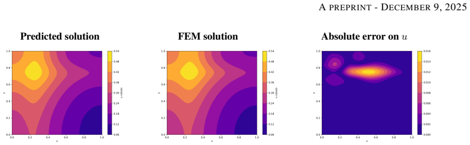
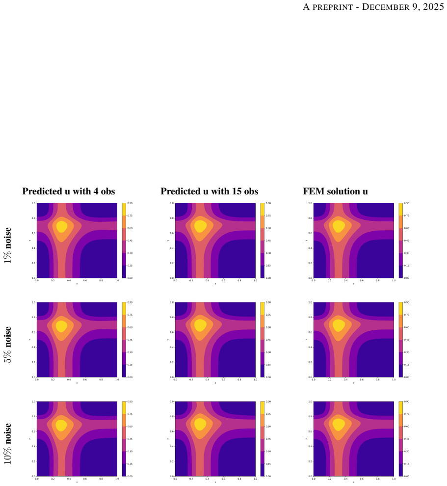
Recent studies have demonstrated the success of deep learning in solving forward and inverse problems in engineering and scientific computing domains, such as physics-informed neural networks (PINNs). Source inversion problems under sparse measurements for parabolic partial differential equations (PDEs) are particularly challenging to solve using PINNs, due to their severe ill-posedness and the multiple unknowns involved including the source function and the PDE parameters. Although the neural tangent kernel (NTK) of PINNs has been widely used in forward problems involving a single neural network, its extension to inverse problems involving multiple neural networks remains less explored. In this work, we propose a weighted adaptive approach based on the NTK of PINNS including multiple separate networks representing the solution, the unknown source, and the PDE parameters. The key idea behind our methodology is to simultaneously solve the joint recovery of the solution, the source function along with the unknown parameters thereby using the underlying partial differential equation as a constraint that couples multiple unknown functional parameters, leading to more efficient use of the limited information in the measurements. We apply our method on the advection-diffusion equation and we present various 2D and 3D numerical experiments using different types of measurements data that reflect practical engineering systems. Our proposed method is successful in estimating the unknown source function, the velocity and diffusion parameters as well as recovering the solution of the equation, while remaining robust to additional noise in the measurements.

Editorial analysis

A structured set of objections, weighed in public.

Desk editor's note, referee report, simulated authors' rebuttal, and a circularity audit. Tearing a paper down is the easy half of reading it; the pith above is the substance, this is the friction.

Desk Editor's Note private letter to a colleague

Multi-network PINN with NTK weighting handles joint source and parameter recovery in advection-diffusion but the experiments stay light on hard numbers and uniqueness checks.

read the letter

The main point is a setup that trains separate networks for the solution u, the source f, and the unknown velocity and diffusion coefficients, then balances their losses with an adaptive NTK scheme. The PDE residual couples everything so the method can work from sparse point measurements on the advection-diffusion equation in 2D and 3D, including cases with added noise. That joint-recovery framing is the concrete step beyond single-network PINNs that have already been tried on forward or simpler inverse problems. The experiments cover several practical measurement patterns, which is helpful for readers who face similar data limitations in fluids or environmental applications. The approach is straightforward to implement once the loss weighting is in place, and the reported robustness to noise is at least directionally encouraging. The main weakness is that the results are described mostly in qualitative terms. There are no tabulated error norms, no baseline comparisons against other inversion techniques, and no explicit test that rules out trade-offs where the source network absorbs mistakes in the parameter networks. The stress-test worry about degeneracy under truly sparse data therefore still needs a direct answer; if the paper only shows that some combination fits the measurements, the claim of reliable joint estimation is only partly supported. This paper is aimed at people already working with PINNs on parabolic inverse problems who need to recover both a distributed source and a few scalar coefficients at the same time. A reader who wants a working template for that setting can extract useful implementation details even if they later tighten the validation themselves. I would send it to peer review because the core construction is sound and the target problem is genuinely hard; the experiments just need more quantitative grounding to match the strength of the method.

Referee Report

2 major / 2 minor

Summary. The paper proposes an extension of physics-informed neural networks (PINNs) that employs adaptive neural tangent kernel (NTK) weighting across multiple separate networks to jointly recover the solution u, unknown source function f, velocity v, and diffusion coefficient D for the advection-diffusion equation from sparse and noisy measurements. The PDE residual serves as the coupling constraint. The approach is tested on various 2D and 3D synthetic cases with different measurement types, claiming successful recovery and noise robustness.

Significance. If the joint inversion proves reliable, the method could advance practical inverse problems for advection-diffusion systems in engineering by making efficient use of limited data through the PDE constraint. The extension of NTK-based adaptive weighting to multi-network inverse settings is a clear technical contribution, and the reproducible numerical experiments on standard test problems add value.

major comments (2)

[Abstract and §4] Abstract and §4 (Numerical Experiments): the central claim of successful estimation of the source, velocity, diffusion parameters, and solution with noise robustness is stated without any quantitative error metrics (e.g., relative L2 errors for f, v, D), baseline comparisons against standard PINNs or other inversion techniques, or details on how post-training validation was performed. This leaves the experimental support for the joint-recovery claim only partially substantiated.
[§3.2] §3.2 (NTK weighting for multi-network PINNs): the adaptive NTK loss weighting is presented as producing a well-conditioned landscape that couples the unknowns and recovers the source despite ill-posedness. However, no ablation or conditioning analysis is provided to show that the weighting prevents the source term from absorbing errors in the parameter networks when measurements are sparse and noisy, which is load-bearing for the claim that the method remains robust under the severe ill-posedness described in the introduction.

minor comments (2)

[§3] Notation for the separate networks (u-network, f-network, parameter networks) is introduced without a consolidated table of symbols, which would improve readability.
[§4] Figure captions in §4 could explicitly state the noise level and number of measurement points for each panel to allow direct comparison across experiments.

Simulated Author's Rebuttal

2 responses · 0 unresolved

We thank the referee for the constructive feedback and detailed comments on our manuscript. We have revised the paper to strengthen the quantitative support for our claims and to provide additional analysis of the NTK weighting. Below we address each major comment point by point.

read point-by-point responses

Referee: [Abstract and §4] Abstract and §4 (Numerical Experiments): the central claim of successful estimation of the source, velocity, diffusion parameters, and solution with noise robustness is stated without any quantitative error metrics (e.g., relative L2 errors for f, v, D), baseline comparisons against standard PINNs or other inversion techniques, or details on how post-training validation was performed. This leaves the experimental support for the joint-recovery claim only partially substantiated.

Authors: We agree that quantitative metrics and baselines would strengthen the experimental support. In the revised manuscript we have added tables of relative L2 errors for the recovered source f, velocity v, diffusion D, and solution u across all 2D and 3D cases. We have also included direct comparisons against a standard single-network PINN and a non-adaptive multi-network variant, together with explicit details on how validation errors were computed on held-out points and the exact noise levels and sparsity patterns used. revision: yes
Referee: [§3.2] §3.2 (NTK weighting for multi-network PINNs): the adaptive NTK loss weighting is presented as producing a well-conditioned landscape that couples the unknowns and recovers the source despite ill-posedness. However, no ablation or conditioning analysis is provided to show that the weighting prevents the source term from absorbing errors in the parameter networks when measurements are sparse and noisy, which is load-bearing for the claim that the method remains robust under the severe ill-posedness described in the introduction.

Authors: We acknowledge that an explicit ablation and conditioning analysis would better substantiate the role of adaptive NTK weighting under ill-posed conditions. We have added a new subsection in the revised §3.2 that reports (i) an ablation comparing recovery accuracy with and without adaptive weighting at increasing sparsity and noise levels, and (ii) the condition-number evolution of the multi-network NTK matrix, showing that the adaptive scheme keeps the loss landscape better balanced and reduces error absorption into the source network. revision: yes

Circularity Check

0 steps flagged

No significant circularity: multi-network PINN-NTK approach validated empirically on standard test cases

full rationale

The paper extends established PINN and NTK weighting techniques to a multi-network setup for joint source-parameter estimation in advection-diffusion PDEs. The derivation consists of defining separate networks for u, f, and parameters, constructing a composite loss with PDE residual and data terms, and applying adaptive NTK-based reweighting; success is then shown via numerical experiments on 2D/3D advection-diffusion problems with sparse/noisy measurements. No load-bearing step reduces by construction to a fitted parameter renamed as prediction, nor does any central claim rest on a self-citation chain that is itself unverified. The reported recovery of source, velocity, and diffusion therefore remains an independent empirical outcome rather than a tautology.

Axiom & Free-Parameter Ledger

0 free parameters · 1 axioms · 0 invented entities

The central claim rests on the standard assumption that the advection-diffusion PDE is an accurate model of the underlying physics and that neural networks have sufficient capacity to represent the solution, source, and parameters simultaneously. No new free parameters or invented entities are introduced beyond the usual neural network weights and the adaptive weighting scheme whose exact form is not detailed in the abstract.

axioms (1)

domain assumption The advection-diffusion PDE is an accurate description of the physical system under study.
The method uses the PDE as the hard constraint that couples the unknown solution, source, and parameters.

pith-pipeline@v0.9.0 · 5568 in / 1334 out tokens · 77434 ms · 2026-05-17T00:02:53.339214+00:00 · methodology

discussion (0)

Lean theorems connected to this paper

Citations machine-checked in the Pith Canon. Every link opens the source theorem in the public Lean library.

IndisputableMonolith/Cost/FunctionalEquation.lean washburn_uniqueness_aczel unclear

?

unclear
Relation between the paper passage and the cited Recognition theorem.

weighted adaptive method based on the neural tangent kernel... multiple separate networks representing the solution, the unknown source, and the PDE parameters

What do these tags mean?

matches: The paper's claim is directly supported by a theorem in the formal canon.
supports: The theorem supports part of the paper's argument, but the paper may add assumptions or extra steps.
extends: The paper goes beyond the formal theorem; the theorem is a base layer rather than the whole result.
uses: The paper appears to rely on the theorem as machinery.
contradicts: The paper's claim conflicts with a theorem or certificate in the canon.
unclear: Pith found a possible connection, but the passage is too broad, indirect, or ambiguous to say the theorem truly supports the claim.

Reference graph

Works this paper leans on

49 extracted references · 49 canonical work pages · 2 internal anchors

[1]

A deep learning framework for solving forward and inverse problems involving nonlinear partial differential equations.J

M Raissi, P Perdikaris, and GE Karniadakis. A deep learning framework for solving forward and inverse problems involving nonlinear partial differential equations.J. Comput. Phys, 378:686–707, 2019

work page 2019
[2]

Physics- informed machine learning.Nature Reviews Physics, 3(6):422–440, 2021

George Em Karniadakis, Ioannis G Kevrekidis, Lu Lu, Paris Perdikaris, Sifan Wang, and Liu Yang. Physics- informed machine learning.Nature Reviews Physics, 3(6):422–440, 2021. 14 APREPRINT- DECEMBER9, 2025

work page 2021
[3]

Gradient-enhanced physics-informed neural networks for forward and inverse pde problems.Computer Methods in Applied Mechanics and Engineering, 393:114823, 2022

Jeremy Yu, Lu Lu, Xuhui Meng, and George Em Karniadakis. Gradient-enhanced physics-informed neural networks for forward and inverse pde problems.Computer Methods in Applied Mechanics and Engineering, 393:114823, 2022

work page 2022
[4]

Annealed adaptive importance sampling method in pinns for solving high dimensional partial differential equations.Journal of Computational Physics, 521:113561, 2025

Zhengqi Zhang, Jing Li, and Bin Liu. Annealed adaptive importance sampling method in pinns for solving high dimensional partial differential equations.Journal of Computational Physics, 521:113561, 2025

work page 2025
[5]

Tackling the curse of dimensionality with physics-informed neural networks.Neural Networks, 176:106369, August 2024

Zheyuan Hu, Khemraj Shukla, George Em Karniadakis, and Kenji Kawaguchi. Tackling the curse of dimensionality with physics-informed neural networks.Neural Networks, 176:106369, August 2024

work page 2024
[6]

Geoffrey Ingram Taylor. I. eddy motion in the atmosphere.Philosophical Transactions of the Royal Society of London. Series A, Containing Papers of a Mathematical or Physical Character, 215(523-537):1–26, 1915

work page 1915
[7]

John Wiley & Sons, 2016

John H Seinfeld and Spyros N Pandis.Atmospheric chemistry and physics: from air pollution to climate change. John Wiley & Sons, 2016

work page 2016
[8]

Source characterization of atmospheric releases using stochastic search and regularized gradient optimization.Inverse Problems in Science and Engineering, 19(8):1097–1124, 2011

B Addepalli, K Sikorski, ER Pardyjak, and MS Zhdanov. Source characterization of atmospheric releases using stochastic search and regularized gradient optimization.Inverse Problems in Science and Engineering, 19(8):1097–1124, 2011

work page 2011
[9]

An adaptive monte carlo markov chain method applied to the flow involving self-similar processes in porous media.Journal of Porous Media, 17(3), 2014

Juarez Azevedo, Gildeberto S Cardoso, and Leizer Schnitman. An adaptive monte carlo markov chain method applied to the flow involving self-similar processes in porous media.Journal of Porous Media, 17(3), 2014

work page 2014
[10]

Simultaneous model calibration and source inversion in atmospheric dispersion models.Pure and Applied Geophysics, 178:757–776, 2021

Juan G García, Bamdad Hosseini, and John M Stockie. Simultaneous model calibration and source inversion in atmospheric dispersion models.Pure and Applied Geophysics, 178:757–776, 2021

work page 2021
[11]

Bayesian estimation of airborne fugitive emissions using a gaussian plume model.Atmospheric Environment, 141:122–138, 2016

Bamdad Hosseini and John M Stockie. Bayesian estimation of airborne fugitive emissions using a gaussian plume model.Atmospheric Environment, 141:122–138, 2016

work page 2016
[12]

Estimating airborne particulate emissions using a finite-volume forward solver coupled with a bayesian inversion approach.Computers & Fluids, 154:27–43, 2017

Bamdad Hosseini and John M Stockie. Estimating airborne particulate emissions using a finite-volume forward solver coupled with a bayesian inversion approach.Computers & Fluids, 154:27–43, 2017

work page 2017
[13]

Bayesian pollution source identification via an inverse physics model.Computational Statistics & Data Analysis, 134:76–92, 2019

Youngdeok Hwang, Hang J Kim, Won Chang, Kyongmin Yeo, and Yongku Kim. Bayesian pollution source identification via an inverse physics model.Computational Statistics & Data Analysis, 134:76–92, 2019

work page 2019
[14]

Shankar Rao

K. Shankar Rao. Source estimation methods for atmospheric dispersion.Atmospheric Environment, 41(33):6964–6973, October 2007

work page 2007
[15]

Cambridge University Press, 2002

Ian G Enting.Inverse problems in atmospheric constituent transport. Cambridge University Press, 2002

work page 2002
[16]

Hengartner, Margaret B

Inanc Senocak, Nicolas W. Hengartner, Margaret B. Short, and W. Brent Daniel. Stochastic event reconstruction of atmospheric contaminant dispersion using bayesian inference.Atmospheric Environment, 42(33):7718–7727, October 2008

work page 2008
[17]

Stochastic reconstruction of multiple source atmospheric contaminant dispersion events.Atmospheric Environment, 74:45–51, August 2013

Derek Wade and Inanc Senocak. Stochastic reconstruction of multiple source atmospheric contaminant dispersion events.Atmospheric Environment, 74:45–51, August 2013

work page 2013
[18]

Tikhonov-type regularization and the finite element method applied to point source estimation in the atmosphere.Atmospheric Environment, 211:69–78, 2019

Roseane AS Albani and Vinicius VL Albani. Tikhonov-type regularization and the finite element method applied to point source estimation in the atmosphere.Atmospheric Environment, 211:69–78, 2019

work page 2019
[19]

An accurate strategy to retrieve multiple source emissions in the atmosphere.Atmospheric Environment, 233:117579, 2020

Roseane AS Albani and Vinicius VL Albani. An accurate strategy to retrieve multiple source emissions in the atmosphere.Atmospheric Environment, 233:117579, 2020

work page 2020
[20]

Uncertainty quantification and atmospheric source estimation with a discrepancy-based and a state-dependent adaptative mcmc.Environmental Pollution, 290:118039, 2021

Roseane AS Albani, Vinicius VL Albani, Hélio S Migon, and Antônio J Silva Neto. Uncertainty quantification and atmospheric source estimation with a discrepancy-based and a state-dependent adaptative mcmc.Environmental Pollution, 290:118039, 2021

work page 2021
[21]

Source area identification with observation from limited monitor sites for air pollution episodes in industrial parks.Atmospheric Environment, 122:1–9, 2015

Zihan Huang, Yuan Wang, Qi Yu, Weichun Ma, Yan Zhang, and Limin Chen. Source area identification with observation from limited monitor sites for air pollution episodes in industrial parks.Atmospheric Environment, 122:1–9, 2015

work page 2015
[22]

Review of physics-informed machine-learning inversion of geophysical data.Geophysics, 89(6):T337–T356, 2024

Gerard T Schuster, Yuqing Chen, and Shihang Feng. Review of physics-informed machine-learning inversion of geophysical data.Geophysics, 89(6):T337–T356, 2024

work page 2024
[23]

Physics-informed neural networks (pinns) for wave propagation and full waveform inversions.Journal of Geophysical Research: Solid Earth, 127(5):e2021JB023120, 2022

Majid Rasht-Behesht, Christian Huber, Khemraj Shukla, and George Em Karniadakis. Physics-informed neural networks (pinns) for wave propagation and full waveform inversions.Journal of Geophysical Research: Solid Earth, 127(5):e2021JB023120, 2022

work page 2022
[24]

Ivan Depina, Saket Jain, Sigurdur Mar Valsson, and Hrvoje Gotovac. Application of physics-informed neural networks to inverse problems in unsaturated groundwater flow.Georisk: Assessment and Management of Risk for Engineered Systems and Geohazards, 16(1):21–36, 2022

work page 2022
[25]

Wavefield reconstruction inversion via physics-informed neural networks

Chao Song and Tariq A Alkhalifah. Wavefield reconstruction inversion via physics-informed neural networks. IEEE Transactions on Geoscience and Remote Sensing, 60:1–12, 2021. 15 APREPRINT- DECEMBER9, 2025

work page 2021
[26]

Microseismic source imaging using physics-informed neural networks with hard constraints.IEEE Transactions on Geoscience and Remote Sensing, 62:1–11, 2024

Xinquan Huang and Tariq A Alkhalifah. Microseismic source imaging using physics-informed neural networks with hard constraints.IEEE Transactions on Geoscience and Remote Sensing, 62:1–11, 2024

work page 2024
[27]

A review of physics informed neural networks for multiscale analysis and inverse problems.Multiscale Science and Engineering, 6(1):1–11, 2024

Dongjin Kim and Jaewook Lee. A review of physics informed neural networks for multiscale analysis and inverse problems.Multiscale Science and Engineering, 6(1):1–11, 2024

work page 2024
[28]

Physics-informed neural networks for inverse problems in supersonic flows.Journal of Computational Physics, 466:111402, 2022

Ameya D Jagtap, Zhiping Mao, Nikolaus Adams, and George Em Karniadakis. Physics-informed neural networks for inverse problems in supersonic flows.Journal of Computational Physics, 466:111402, 2022

work page 2022
[29]

Solving forward and inverse problems of contact mechanics using physics-informed neural networks.Advanced Modeling and Simulation in Engineering Sciences, 11(1):11, 2024

Tarik Sahin, Max von Danwitz, and Alexander Popp. Solving forward and inverse problems of contact mechanics using physics-informed neural networks.Advanced Modeling and Simulation in Engineering Sciences, 11(1):11, 2024

work page 2024
[30]

Physics-informed learning of governing equations from scarce data.Nature communications, 12(1):6136, 2021

Zhao Chen, Yang Liu, and Hao Sun. Physics-informed learning of governing equations from scarce data.Nature communications, 12(1):6136, 2021

work page 2021
[31]

Data- efficient kernel methods for learning differential equations and their solution operators: Algorithms and error analysis.arXiv preprint arXiv:2503.01036, 2025

Yasamin Jalalian, Juan Felipe Osorio Ramirez, Alexander Hsu, Bamdad Hosseini, and Houman Owhadi. Data- efficient kernel methods for learning differential equations and their solution operators: Algorithms and error analysis.arXiv preprint arXiv:2503.01036, 2025

work page arXiv 2025
[32]

Data-efficient kernel methods for learning hamiltonian systems.arXiv preprint arXiv:2509.17154, 2025

Yasamin Jalalian, Mostafa Samir, Boumediene Hamzi, Peyman Tavallali, and Houman Owhadi. Data-efficient kernel methods for learning hamiltonian systems.arXiv preprint arXiv:2509.17154, 2025

work page arXiv 2025
[33]

Data-driven discovery of partial differential equations.Science advances, 3(4):e1602614, 2017

Samuel H Rudy, Steven L Brunton, Joshua L Proctor, and J Nathan Kutz. Data-driven discovery of partial differential equations.Science advances, 3(4):e1602614, 2017

work page 2017
[34]

Understanding and mitigating gradient flow pathologies in physics-informed neural networks.SIAM Journal on Scientific Computing, 43(5):A3055–A3081, 2021

Sifan Wang, Yujun Teng, and Paris Perdikaris. Understanding and mitigating gradient flow pathologies in physics-informed neural networks.SIAM Journal on Scientific Computing, 43(5):A3055–A3081, 2021

work page 2021
[35]

A dual-dimer method for training physics-constrained neural networks with minimax architecture.Neural Networks, 136:112–125, 2021

Dehao Liu and Yan Wang. A dual-dimer method for training physics-constrained neural networks with minimax architecture.Neural Networks, 136:112–125, 2021

work page 2021
[36]

Solving allen-cahn and cahn-hilliard equations using the adaptive physics informed neural networks.arXiv preprint arXiv:2007.04542, 2020

Colby L Wight and Jia Zhao. Solving allen-cahn and cahn-hilliard equations using the adaptive physics informed neural networks.arXiv preprint arXiv:2007.04542, 2020

work page arXiv 2007
[37]

Self-adaptive physics-informed neural networks using a soft attention mechanism

Levi McClenny Ulisses Braga-Neto. Self-adaptive physics-informed neural networks using a soft attention mechanism. 2021

work page 2021
[38]

When and why pinns fail to train: A neural tangent kernel perspective.Journal of Computational Physics, 449:110768, 2022

Sifan Wang, Xinling Yu, and Paris Perdikaris. When and why pinns fail to train: A neural tangent kernel perspective.Journal of Computational Physics, 449:110768, 2022

work page 2022
[39]

Neural tangent kernel: Convergence and generalization in neural networks.Advances in neural information processing systems, 31, 2018

Arthur Jacot, Franck Gabriel, and Clément Hongler. Neural tangent kernel: Convergence and generalization in neural networks.Advances in neural information processing systems, 31, 2018

work page 2018
[40]

Sifan Wang, Hanwen Wang, and Paris Perdikaris. On the eigenvector bias of fourier feature networks: From regression to solving multi-scale pdes with physics-informed neural networks.Computer Methods in Applied Mechanics and Engineering, 384:113938, 2021

work page 2021
[41]

Neural tangent kernel analysis to probe convergence in physics-informed neural solvers: Pikans vs

Salah A Faroughi and Farinaz Mostajeran. Neural tangent kernel analysis to probe convergence in physics-informed neural solvers: Pikans vs. pinns.arXiv preprint arXiv:2506.07958, 2025

work page arXiv 2025
[42]

Cambridge University Press, 2001

Dietrich Braess.Finite elements: Theory, fast solvers, and applications in solid mechanics. Cambridge University Press, 2001

work page 2001
[43]

SIAM, 2004

John C Strikwerda.Finite difference schemes and partial differential equations. SIAM, 2004

work page 2004
[44]

Physics Informed Deep Learning (Part I): Data-driven Solutions of Nonlinear Partial Differential Equations

Maziar Raissi, Paris Perdikaris, and George Em Karniadakis. Physics informed deep learning (part i): Data-driven solutions of nonlinear partial differential equations.arXiv preprint arXiv:1711.10561, 2017

work page internal anchor Pith review Pith/arXiv arXiv 2017
[45]

Deepxde: A deep learning library for solving differential equations.SIAM review, 63(1):208–228, 2021

Lu Lu, Xuhui Meng, Zhiping Mao, and George Em Karniadakis. Deepxde: A deep learning library for solving differential equations.SIAM review, 63(1):208–228, 2021

work page 2021
[46]

The mathematics of atmospheric dispersion modeling.Siam Review, 53(2):349–372, 2011

John M Stockie. The mathematics of atmospheric dispersion modeling.Siam Review, 53(2):349–372, 2011

work page 2011
[47]

Analytical solutions of the atmospheric diffusion equation with multiple sources and height-dependent wind speed and eddy diffusivities.Atmospheric Environment, 30(2):239–254, 1996

Jin-Sheng Lin and Lynn M Hildemann. Analytical solutions of the atmospheric diffusion equation with multiple sources and height-dependent wind speed and eddy diffusivities.Atmospheric Environment, 30(2):239–254, 1996

work page 1996
[48]

Airborne contaminant source estimation using a finite-volume forward solver coupled with a Bayesian inversion approach

Bamdad Hosseini and John M Stockie. Airborne contaminant source estimation using a finite-volume forward solver coupled with a bayesian inversion approach.arXiv preprint arXiv:1607.03518, 2016

work page internal anchor Pith review Pith/arXiv arXiv 2016
[49]

Oxford University Press New York, 1999

S Pal Arya et al.Air pollution meteorology and dispersion, volume 310. Oxford University Press New York, 1999. 16 APREPRINT- DECEMBER9, 2025 A Proof of lemma1 Proof 1We recall the loss function to minimize: L(ΘΘΘ) =λ rLr(ΘΘΘ) +λ bLb(θuθuθu) +λ zLz(θuθuθu),Θ ΘΘ ={θ uθuθu, θfθfθf , γ}(12) and the gradient flow system dΘΘΘ(s) ds =−∇ ΘΘΘL(ΘΘΘ(s)),withΘ ΘΘ(s) ...

work page 1999