Back-action from inertial and non-inertial Unruh-DeWitt detectors revisited in covariant perturbation theory
Pith reviewed 2026-05-16 21:49 UTC · model grok-4.3
The pith
The energy flux from the field's stress-energy tensor exactly balances the energy transitions of Unruh-DeWitt detectors for both inertial and accelerated motion.
A machine-rendered reading of the paper's core claim, the machinery that carries it, and where it could break.
Core claim
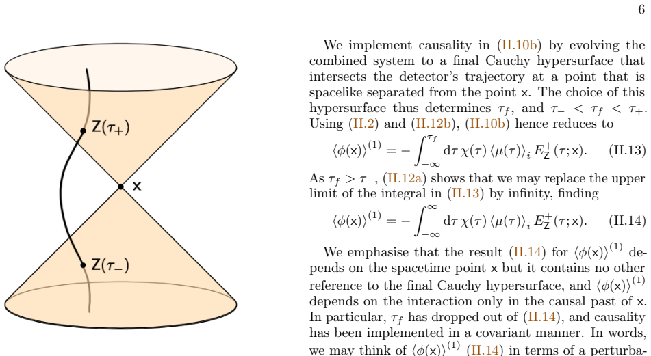
The central claim is that the renormalized expectation value of the field's stress-energy tensor around an inertial or uniformly accelerated Unruh-DeWitt detector yields energy fluxes that exactly compensate the detector's internal energy changes arising from its interactions with vacuum fluctuations. This exact accounting holds without conditioning on measurement outcomes and applies to detectors switched on in the asymptotic past, with the fluctuating part of the detector's correlations fully determining the back-action for an energy-eigenstate preparation.
What carries the argument
The manifestly causal two-point function of the detector-field system obtained in second-order covariant perturbation theory, from which the expectation value of the stress-energy tensor is constructed.
Load-bearing premise
The field begins in a zero-mean Gaussian Hadamard state and the detector-field interaction is treated perturbatively only to second order without any conditioning on detector measurement outcomes.
What would settle it
A numerical or analytic evaluation of the integrated energy flux from the stress-energy tensor that fails to equal the detector's energy change for a specific uniformly accelerated trajectory switched on in the past would falsify the exact balance.
Figures


read the original abstract
We investigate the back-action from a spatially pointlike particle detector on a quantum scalar field, as characterised by the expectation value of the field's stress-energy tensor, without conditioning on a measurement of the detector. First, assuming the field to be initially in a zero-mean Gaussian Hadamard state in a globally hyperbolic spacetime, we evaluate the field's two-point function in second-order perturbation theory by techniques of covariant curved spacetime quantum field theory, which allow a full control of the time and space localisation of the interaction, and do not rely on field mode decompositions or non-local particle countings. The detector's two-point function splits into a deterministic and a fluctuating part, and we show that this split is maintained in the back-action. We then specialise to a two-level Unruh-DeWitt detector, prepared in an energy eigenstate, for which the back-action is fully fluctuating. We compute the renormalised stress-energy tensor for a massless scalar field in $(3+1)$-dimensional Minkowski spacetime for a general detector trajectory, using the manifestly causal two-point function. We present explicit analytic and numerical results for an inertial detector and a uniformly linearly accelerated detector, switched on in the asymptotic past. The energy flux into and out of the accelerated detector accounts exactly for the energy gained and lost by the detector in its transitions due to the Unruh effect. The same holds for the outward flux associated with de-excitations of the inertial detector, which has a vanishing excitation rate and no inward flux. A novelty with the accelerated detector is two regions of negative energy density when the detector is initially prepared in its ground state, one near the Rindler horizon that bounds the causal future of the trajectory, the other in the far future of the trajectory.
Editorial analysis
A structured set of objections, weighed in public.
Referee Report
Summary. The paper computes the back-action of a pointlike Unruh-DeWitt detector on a quantum scalar field via the renormalized expectation value of the stress-energy tensor, using second-order covariant perturbation theory in globally hyperbolic spacetimes. The field's two-point function is constructed manifestly causally from a zero-mean Gaussian Hadamard state without mode expansions. For a two-level detector in Minkowski space, the back-action is shown to be fully fluctuating when the detector starts in an energy eigenstate. Explicit analytic and numerical results for inertial and uniformly accelerated trajectories (switched on in the asymptotic past) demonstrate that the integrated energy fluxes into/out of the detector exactly equal the net energy change from Unruh-induced transitions. A new feature is the appearance of two regions of negative energy density for an accelerated detector prepared in its ground state.
Significance. If the central results hold, the work supplies a consistent, mode-independent verification that energy is conserved between the detector and the field in the Unruh setting, obtained from a manifestly causal two-point function and standard Hadamard renormalization. The exact flux-transition balance constitutes a non-trivial internal check of the perturbative framework. The reported negative-energy-density regions constitute a concrete, falsifiable prediction that can be tested in future calculations with different switching functions or trajectories. The approach avoids non-local particle interpretations and is therefore directly extensible to curved spacetimes.
major comments (1)
- [§4.3] §4.3, around Eq. (35): the exact equality between the integrated flux and the detector energy change is demonstrated numerically for the specific asymptotic-past switching; an analytic identity showing that the equality holds for arbitrary compactly supported switching functions would make the claim independent of the particular regularization of the interaction.
minor comments (3)
- [Abstract] Abstract: the phrase 'manifestly causal two-point function' is used without a one-sentence definition; a brief parenthetical reference to the point-splitting construction employed would aid readers unfamiliar with the covariant formalism.
- [Figures 2 and 4] Figure 2 (inertial case) and Figure 4 (accelerated case): the color scale for the renormalized energy density does not indicate the location of the Rindler horizon or the light-cone boundaries; adding these reference lines would clarify the spatial support of the negative-energy regions.
- [§2.1] §2.1: the notation for the detector-field coupling constant and the switching function is introduced without an explicit statement of their dimensions; a short remark on units would prevent confusion when comparing to other Unruh-DeWitt literature.
Simulated Author's Rebuttal
We thank the referee for their positive assessment and constructive suggestion. We address the single major comment below.
read point-by-point responses
-
Referee: [§4.3] §4.3, around Eq. (35): the exact equality between the integrated flux and the detector energy change is demonstrated numerically for the specific asymptotic-past switching; an analytic identity showing that the equality holds for arbitrary compactly supported switching functions would make the claim independent of the particular regularization of the interaction.
Authors: We agree that the numerical verification is performed for the standard asymptotic-past switching, which is chosen to suppress transient effects. The equality itself follows directly from the structure of the second-order two-point function constructed via covariant perturbation theory and the definition of the renormalized stress-energy tensor; this construction is causal and does not rely on mode expansions. While an explicit analytic identity valid for arbitrary compactly supported switching would indeed strengthen independence from regularization details, obtaining it requires a more general analysis of the time-ordered products that lies outside the present scope. In the revised manuscript we will insert a short clarifying paragraph in §4.3 that explains the origin of the equality within our framework and states that the numerical check for the conventional switching constitutes a non-trivial internal consistency test. This constitutes a partial revision. revision: partial
Circularity Check
No significant circularity; derivation is self-contained
full rationale
The paper computes the field's two-point function via standard second-order covariant perturbation theory in a Hadamard state, using manifestly causal techniques that do not rely on mode decompositions or particle counting. The renormalised stress-energy tensor is obtained by subtracting the vacuum contribution, and the energy-flux accounting for detector transitions follows as an explicit verification from the resulting expressions for inertial and accelerated trajectories. No parameters are fitted to the target fluxes, no self-definitional loops appear in the split into deterministic/fluctuating parts, and the Unruh effect enters only as an external benchmark rather than a load-bearing self-citation. The central claims therefore reduce to the perturbative expansion and the known two-point function structure, without circular reduction to the paper's own inputs.
Axiom & Free-Parameter Ledger
axioms (1)
- domain assumption Field initially in a zero-mean Gaussian Hadamard state in a globally hyperbolic spacetime
Lean theorems connected to this paper
-
IndisputableMonolith/Cost/FunctionalEquation.leanwashburn_uniqueness_aczel unclear?
unclearRelation between the paper passage and the cited Recognition theorem.
The energy flux into and out of the accelerated detector accounts exactly for the energy gained and lost by the detector in its transitions due to the Unruh effect.
-
IndisputableMonolith/Foundation/RealityFromDistinction.leanreality_from_one_distinction unclear?
unclearRelation between the paper passage and the cited Recognition theorem.
We evaluate the field’s two-point function in second-order perturbation theory by techniques of covariant curved spacetime quantum field theory
What do these tags mean?
- matches
- The paper's claim is directly supported by a theorem in the formal canon.
- supports
- The theorem supports part of the paper's argument, but the paper may add assumptions or extra steps.
- extends
- The paper goes beyond the formal theorem; the theorem is a base layer rather than the whole result.
- uses
- The paper appears to rely on the theorem as machinery.
- contradicts
- The paper's claim conflicts with a theorem or certificate in the canon.
- unclear
- Pith found a possible connection, but the passage is too broad, indirect, or ambiguous to say the theorem truly supports the claim.
Forward citations
Cited by 1 Pith paper
-
Relativistic single-electron wavepacket in quantum electromagnetic fields II: Quantum radiation emitted by a uniformly accelerated electron
Quantum radiation from a single-electron wavepacket at rest vanishes exactly, while for a uniformly accelerated electron the radiated power shows secular growth in the long-time regime with a classical interpretation,...
Reference graph
Works this paper leans on
-
[1]
Energy density Figure 5 shows a plot ofξ−2 ⟨Tηη ⟩(2) as a function of aξ and E/a, evaluated from(VI.6a). This is the energy density seen by the observers on the uniformly accelerated worldlines of constantξ. 15 0 1 2 aξ −4 −2 0 2 4 E/a −100 −10−2 0 10−2 100 102 104 FIG. 5. a−4ξ−2 ⟨Tηη ⟩(2) as a function ofaξ and E/a, obtained from (VI.6a). At the detector...
-
[2]
Energy flux Figure 6 shows a plot ofξ−1 ⟨Tηξ⟩(2), in the plane of the detector’s wordline, evaluated from(VI.6b). The energy flux in the direction of increasingξ seen by an observer at constant ξ is equal to−ξ−1 ⟨Tηξ⟩(2) (cf. the discussion in Section VC for the inertial detector trajectory). For de-excitations, E < 0, the direction of the flux is away fr...
-
[3]
This is the energy density seen by the Milne observers
Energy density Figure 8 shows a plot of⟨Tσσ ⟩(2) (VI.9a) as a function of aσ and E/a. This is the energy density seen by the Milne observers. At the Milne infinityaσ→ ∞ , in the far future, the leading term in the falloff of⟨Tσσ ⟩(2) consists of terms proportional to σ−6 and to the real and imaginary parts of σ−6(aσ)2iE/a, with E-dependent coefficients, a...
-
[4]
This region of negative energy density for largeσ and E is visible in Figure 8, including the asymptotic behaviour where the zero-crossing approaches aσ = √ 3 for large positive E. While this region of negative energy density is not com- pact, the σ−6 suppression in the coefficient of1 /E in (VI.19) indicates that the energy density does not take large ne...
-
[5]
Energy flux Figure 9 shows a plot of σ−1 ⟨Tσρ⟩(2), evaluated from (VI.9b). The energy flux in the direction of in- creasing ρ seen by an observer at constantρ is equal to −σ−1 ⟨Tσρ⟩(2). For de-excitation gaps the flux is left-moving, away from the detector, and for excitation gaps the flux is right-moving, towards the detector. This is consistent with the...
-
[6]
10 shows spacetime plots of the Minkowski energy density⟨T tt⟩(2) (VI.2a), for selected values ofE/a
Energy density Fig. 10 shows spacetime plots of the Minkowski energy density⟨T tt⟩(2) (VI.2a), for selected values ofE/a. Close to the detector’s worldline,⟨Ttt⟩(2) is asymptotic to ⟨Ttt⟩(2) ∼ a2 v2 +u 2 64π2√−uv−a −1 4 ,(VI.21) where we recall that the detector’s worldline is atuv = −a−2 with u < 0and v > 0, we have used 3.911.2 in [96] in the first inte...
-
[7]
The energy flux in the direction of increasingzas seen by a static Minkowski observer is − ⟨Ttz⟩(2)
Energy flux Figure 11 shows spacetime plots of⟨Ttz⟩(2) (VI.2b), for selected values ofE/a. The energy flux in the direction of increasingzas seen by a static Minkowski observer is − ⟨Ttz⟩(2). A striking feature in Figure 11 is the qualitative dif- −4 −2 0 2 4 at E/a = −3 E/a = 3 −4 −2 0 2 4 at E/a = −1 E/a = 1 −2.5 0.0 2.5 az −4 −2 0 2 4 at E/a = −0.1 −2....
-
[8]
shows that the second term isO(η−1)as η→ ∞ . The change of variablesv = κ(η)ω puts the third term in the form 1 π2 κ(η)|E| Z κ(η)|E| 0 dv 1−cosv v2 bψ v κ(η) 2 = 1 π2 κ(η)|E| Z ∞ 0 dv 1−cosv v2 bψ v κ(η) 2 − 1 π2 κ(η)|E| Z ∞ κ(η)|E| dv 1−cosv v2 bψ v κ(η) 2 . (A.13) The large argument behaviour ofbψ then implies that as η→ ∞ , the first term in(A.13)∼ τp|...
-
[9]
UDW detector For the UDW detector, in the notation of Section IIIB, (B.2) gives e−iE(τ+τ ′) Cov(σ−, σ−) + e−iE(τ−τ ′) Cov(σ−, σ+) + eiE(τ−τ ′) Cov(σ+, σ−) + eiE(τ+τ ′) Cov(σ+, σ+) = 0. (B.3) If the detector is nondegenerate, E̸ = 0, linear in- dependence of the set {e±iE(τ+τ ′), e±iE(τ−τ ′)} implies that Cov(σ−, σ−) = Cov(σ−, σ+) = Cov(σ+, σ−) = Cov(σ+, σ...
-
[10]
However, we also have Cov(a, a†)−Cov(a †, a) =⟨[a, a †]⟩= 1,(B.6) using[ a, a†] = 1D
HO detector For the HO detector, in the notation of Section IIIC, (B.2) gives e−iΩ(τ+τ ′) Cov(a, a) + e−iΩ(τ−τ ′) Cov(a, a†) + eiΩ(τ−τ ′) Cov(a†, a) + eiΩ(τ+τ ′) Cov(a†, a†) = 0, (B.5) AsΩ > 0by assumption, the set {e±iΩ(τ+τ ′), e±iΩ(τ−τ ′)} islinearlyindependent, and (B.5)impliesthat Cov(a, a) = Cov(a, a†) = Cov(a†, a) = Cov(a†, a†) = 0. However, we also...
-
[11]
Split ofI µν From (IV.11) we recall that ⟨ϕ(x)ϕ(x′)⟩(2) = Im χ(τ−)eiEτ− 4π3f ′(τ−;x) − Z τ− −∞ dτ χ(τ)e −iEτ f(τ;x ′) +iπ χ(τ ′ −)e−iEτ ′ − f ′(τ ′ −;x ′) Θ(τ− −τ ′ −) + (x↔x ′), (C.1) wherexandx ′ are timelike separated and sufficiently close to each other.− R denotes the Cauchy principal value integral in the integral term in which the denominator has a...
-
[12]
Evaluation ofC µν In Cµν (C.3a), evaluating the derivatives and taking the coincidence limit gives Cµν(x,x) =πE 2∂µτ−∂ντ− χ(τ−)2 f ′(τ−;x) 2 +π∂ µ χ(τ−) f ′(τ−;x) ∂ν χ(τ−) f ′(τ−;x) ,(C.4) where we have used that the terms linear inE vanish on taking the real part. To eliminate the derivatives ofτ−, we recall that the equation definingτ− as a function ofx...
-
[13]
Evaluation ofS µν We now turn toSµν (C.3b). In the explicitly displayed term in(C.3b), the contribution from∂µ acting on the τ− at the upper limit of the integral vanishes, on taking the imaginary part, and similarly in the(x↔ x′)term when the primed derivative acts on theτ ′ − at the upper limit of the integral. We can therefore write Sµν(x,x ′) = Im ∂µ ...
-
[14]
Result forI µν Combining (C.9), (C.14), (C.16) and (C.27), the final expression forI µν (IV.12) is Iµν = 1 4π3f ′(τ−) " −E∂τ αµ(τ)α ν(τ) f ′(τ) τ=τ − +π E2αµ(τ−)αν(τ−) +α ′ µ(τ−)α′ ν(τ−) f ′(τ−) −2 Z τ− −∞ dτ E2 sin(E(τ−τ −)) f(τ) α(µ(τ−)αν)(τ) +Ecos(E(τ−τ −)) α′ (µ(τ−)αν)(τ)−α ′ (µ(τ)α ν)(τ−) f(τ) + sin(E(τ−τ −)) f(τ) α′ (µ(τ−)α′ ν)(τ) # ,(C.28) where th...
-
[15]
Alternative expression forI µν We shall give forIµν (C.28) an alternative expression that will be convenient for handling the Rindler trajectory detector in Appendix F. We make the technical assumption thatf(τ)is defined for −∞< τ≤τ −, that is, the trajectory is defined at ar- bitrarily negative proper times in the past. Recalling that f(τ−) = 0, f ′(τ) >...
-
[16]
Null coordinates Recall that in the Minkowski coordinates(t, x, y, z)the Rindler trajectory (VI.1) is given by Z(τ) = 1 a sinh(aτ),0,0, 1 a cosh(aτ) ,(F.1) where the positive constanta is the proper acceleration. In terms of the null coordinatesu = t−z and v = t + z, the squared geodesic distance (IV.6) is f(τ;x) =ua −1eaτ −va −1e−aτ −uv+x 2 +y 2 +a −2, (...
-
[17]
Simplifying⟨T µν ⟩(2) In the expression(C.37) for Iµν, the key simplification for the Rindler trajectory is the identity ˜α′ µ −f ′(τ)β µ(τ) f(τ) =a U˜αµ −A µ ˜f ′ ∂τ 2eaτ− Ve −aτ +Ue aτ− , (F.7) where At = V−U 2V , A z =− V+U 2V , A x =A y = 0,(F.8) which can be verified by a direct calculation, using K=−Ue aτ− +Ve −aτ− .(F.9) In the cosine term in (C.37...
-
[18]
S. A. Fulling, Phys. Rev. D7, 2850 (1973)
work page 1973
-
[19]
P. C. W. Davies, J. Phys. A8, 609 (1975)
work page 1975
-
[20]
W. G. Unruh, Phys. Rev. D14, 870 (1976)
work page 1976
-
[21]
B. S. DeWitt, inGeneral Relativity: an Einstein cen- tenary survey, edited by S. W. Hawking and W. Israel (Cambridge University Press, Cambridge, 1979)
work page 1979
-
[22]
N. D. Birrell and P. C. W. Davies,Quantum Fields in Curved Space, Cambridge Monographs on Mathematical Physics (Cambridge University Press, 1982)
work page 1982
-
[23]
L. C. B. Crispino, A. Higuchi, and G. E. A. Matsas, Rev. Mod. Phys.80, 787 (2008)
work page 2008
-
[24]
S. A. Fulling and G. E. A. Matsas, Scholarpedia9, 31789 (2014), revision #143950
work page 2014
-
[25]
J. R. Letaw, Phys. Rev. D23, 1709 (1981)
work page 1981
- [26]
-
[27]
S. Biermann, S. Erne, C. Gooding, J. Louko, J. Schmied- mayer, W. G. Unruh, and S. Weinfurtner, Phys. Rev. D 102, 085006 (2020)
work page 2020
-
[28]
L. J. A. Parry and J. Louko, Phys. Rev. D111, 025012 (2025)
work page 2025
-
[29]
S. W. Hawking, Commun. Math. Phys.43, 199 (1975), [Erratum: Commun.Math.Phys. 46, 206 (1976)]
work page 1975
-
[30]
J. B. Hartle and S. W. Hawking, Phys. Rev. D13, 2188 (1976)
work page 1976
-
[31]
G. W. Gibbons and S. W. Hawking, Phys. Rev. D15, 2738 (1977)
work page 1977
- [32]
-
[33]
L. H. Ford and C. Pathinayake, Phys. Rev. D39, 3642 (1989)
work page 1989
-
[34]
L. J. Garay, M. Martín-Benito, and E. Martín-Martínez, Phys. Rev. D89, 043510 (2014)
work page 2014
-
[35]
R. H. Jonsson, E. Martin-Martinez, and A. Kempf, Phys. Rev. Lett.114, 110505 (2015)
work page 2015
- [36]
- [37]
-
[38]
A. S. Wilkinson and J. Louko, Phys. Rev. D111, 025008 (2025)
work page 2025
- [39]
- [40]
- [41]
-
[42]
A. Pozas-Kerstjens and E. Martín-Martínez, Phys. Rev. D92, 064042 (2015)
work page 2015
-
[43]
J. Foo, C. S. Arabaci, M. Zych, and R. B. Mann, Phys. Rev. Lett.129, 181301 (2022)
work page 2022
-
[44]
J. Foo, C. S. Arabaci, M. Zych, and R. B. Mann, Phys. Rev. D107, 045014 (2023)
work page 2023
-
[45]
L. Goel, E. A. Patterson, M. R. Preciado-Rivas, M. Tora- bian, R. B. Mann, and N. Afshordi, Phys. Rev. D111, 025015 (2025)
work page 2025
-
[46]
L. C. Barbado, E. Castro-Ruiz, L. Apadula, and Č. Brukner, Phys. Rev. D102, 045002 (2020)
work page 2020
-
[47]
J. Foo, S. Onoe, and M. Zych, Phys. Rev. D102, 085013 (2020)
work page 2020
- [48]
-
[49]
C. J. Fewster and R. Verch, Commun. Math. Phys.378, 851 (2020)
work page 2020
-
[50]
J. Polo-Gómez, L. J. Garay, and E. Martín-Martínez, Phys. Rev. D105, 065003 (2022)
work page 2022
-
[51]
J. Polo-Gómez, T. R. Perche, and E. Martín-Martínez, State updates and useful qubits in relativistic quantum information (2025), arXiv:2506.18906 [quant-ph]
-
[52]
J. J. Bisognano and E. H. Wichmann, J. Math. Phys. 16, 985 (1975)
work page 1975
-
[53]
J. J. Bisognano and E. H. Wichmann, J. Math. Phys. 17, 303 (1976)
work page 1976
-
[54]
G. L. Sewell, Physics Letters A79, 23 (1980)
work page 1980
-
[55]
G. L. Sewell, Annals Phys.141, 201 (1982)
work page 1982
- [56]
-
[57]
W. G. Unruh and R. M. Wald, Phys. Rev. D29, 1047 (1984)
work page 1984
-
[58]
P. G. Grove, Class. Quant. Grav.3, 801 (1986)
work page 1986
- [59]
-
[60]
D. J. Raine, D. W. Sciama, and P. G. Grove, Proc. R. Soc. Lond. A435, 205 (1991)
work page 1991
-
[61]
W. G. Unruh, Phys. Rev. D46, 3271 (1992)
work page 1992
- [62]
- [63]
- [64]
-
[65]
On "the'' electric field of a uniformly accelerating charge
D. Garfinkle, On “the” electric field of a uniformly accel- erating charge (2019), arXiv:1901.04486 [gr-qc]
work page internal anchor Pith review Pith/arXiv arXiv 2019
- [66]
- [67]
-
[68]
G. W. Ford and R. F. O’Connell, Phys. Lett. A350, 17 (2006)
work page 2006
-
[69]
A. Higuchi, G. E. A. Matsas, and D. Sudarsky, Phys. Rev. D45, R3308 (1992)
work page 1992
- [70]
- [71]
-
[72]
F. Portales-Oliva and A. G. S. Landulfo, Phys. Rev. D 106, 065002 (2022)
work page 2022
-
[73]
G. Vacalis, A. Higuchi, R. Bingham, and G. Gregori, Phys. Rev. D109, 024044 (2024)
work page 2024
-
[74]
K. Gallock-Yoshimura, Y. Osawa, and Y. Nambu, Phys. Rev. D111, 105012 (2025)
work page 2025
-
[75]
A. Garcia-Chung, B. A. Juárez-Aubry, and D. Sudarsky, Phys. Rev. D108, 025002 (2023)
work page 2023
- [76]
- [77]
-
[78]
C. J. Fewster and R. Verch, Class. Quant. Grav.30, 235027 (2013)
work page 2013
- [79]
-
[80]
E. Martín-Martínez, M. Montero, and M. del Rey, Phys. Rev. D87, 064038 (2013)
work page 2013
discussion (0)
Sign in with ORCID, Apple, or X to comment. Anyone can read and Pith papers without signing in.