Deep Learning for Accelerated Long-Horizon Forecasting of Multicomponent Multiphase Microstructure Evolution in High-Entropy Alloys

Hamidreza Razavi; Nele Moelans

REVIEW 4 major objections 5 minor 21 references

Deep Learning for Accelerated Long-Horizon Forecasting of Multicomponent Multiphase Microstructure Evolution in High-Entropy Alloys

T0 review · 4 major / 5 minor · reviewed 2026-08-01 · deepseek-v4-flash

Challenge this review Re-run · record.json Download PDF Read on arXiv ↗ Review JSON

Pith's one-line read A latent graph-based AE-GCN-LSTM surrogate can forecast the coupled evolution of four concentration fields and two phases in AlCrFeNi for up to 3,000,000 timesteps with 7,200–62,300× speedups and zero-shot generalization to unseen precipita

desk verdict A promising surrogate architecture for quaternary phase-field evolution, but the headline generalization claims are undermined by the best-match scan on 512x512, a domain-size contradiction, and missing quantitative OOD metrics. read the letter →

arxiv 2607.27820 v1 pith:25XT65BD submitted 2026-07-30 cond-mat.mtrl-sci cs.AIcs.CE

Hamidreza Razavi , Nele Moelans This is my paper · ORCID

classification cond-mat.mtrl-scics.AIcs.CE

keywords phase-fieldsurrogatehigh-entropyalloymicrostructureevolutiongraphneuralnetworkLSTMforecastingzero-shotgeneralizationautoencoderAlCrFeNi

verification ladder T0 review T1 audit T2 compute T3 formal

The pith

A machine-rendered reading of the paper's core claim, the machinery that carries it, and where it could break.

The reading

This paper tries to establish that a neural surrogate can replace a phase-field solver for long-horizon microstructure evolution in a quaternary high-entropy alloy, not just interpolate training data. The authors compress five physical fields (four elemental concentrations plus a phase indicator) into a latent space, represent that space as a graph, and learn the spatiotemporal dynamics with a GCN-LSTM. They then show the trained model forecasts evolution for up to three million simulation timesteps on unseen microstructures, with speedups between about 7,200× and 62,300×. The zero-shot generalization claims extend to unseen precipitate sizes, positions, counts, merging/splitting events, computational domains up to 512×512, and off-nominal alloy compositions. If correct, this offers a path to high-throughput screening of multicomponent alloys without running expensive phase-field simulations.

What carries the argument

The key mechanism is the separation of conserved and non-conserved variables through the entire pipeline. The autoencoder has two decoder branches—one for concentration fields with a conservation constraint, one for the phase-field logits—so that chemical composition and phase morphology are not mixed. In the forecasting GCN-LSTM, orthogonality between the concentration and phase branches further prevents feature leakage. This separation, combined with the graph formulation of latent nodes, is what lets the model transfer to unseen spatial domains and compositions: the learned dynamics are local in space and tied to physical conservation laws.

What would settle it

Run the frozen model on a 512×512 domain with two widely separated precipitates (so that patch boundaries cut through the matrix) and compare the forecast to a fresh phase-field simulation; if visible seams or non-physical concentration gradients appear at patch boundaries, or if the composition conservation loss grows beyond the training value, the locality assumption fails.

Watch

Extended reading notes

Core claim

The central discovery is that a compact latent graph representation suffices to learn the evolution operator of a multicomponent, multiphase system. An autoencoder reduces each five-channel microstructure state to a latent feature map, and each spatial location becomes a node in a graph with four-neighbor connectivity. A GCN stack propagates local spatial information at each time step, and a two-branch LSTM advances the latent state in time: one branch evolves the conserved concentration fields, the other the non-conserved phase-field order parameter. The authors report that this learned dynamics reproduces the dominant phase morphology and compositional evolution for horizons up to 3,000,00

Load-bearing premise

The premise that the latent evolution operator is approximately local, both in space and in composition space, so that patch-based stitching on larger domains and transfer to off-nominal compositions do not introduce errors that accumulate over millions of timesteps.

Editorial extensions

If this is right

Phase-field simulations of multicomponent alloys could be replaced by a learned surrogate for parameter screening and design optimization, cutting simulation time from days to seconds.
The zero-shot generalization to larger domains via overlapping patches indicates that models trained on small simulations can be applied to industrially relevant sample sizes without retraining.
Off-nominal compositions within a few atomic percent are forecastable without retraining, suggesting the latent dynamics encode chemistry-driven evolution rather than memorizing one composition.
Separating conserved and non-conserved fields during compression and forecasting prevents drift in total composition, a prerequisite for physically meaningful long-horizon predictions.
The framework is a natural extension of earlier binary-alloy surrogates, indicating a path toward a general-purpose surrogate for multicomponent systems.

Reading between the lines

Editorial extensions of the paper, not claims the author makes directly.

If the learned latent dynamics are truly local in state space, a single small-domain training set could serve as the foundation for a universal microstructure evolution surrogate across many alloy families; the authors only demonstrate this on one quaternary system, but the architectural choices suggest the claim is testable.
The patch-based transfer to larger domains has an implicit assumption that cross-patch couplings are negligible; systems with long-range elastic or chemical interactions could break this assumption and would require a different stitching strategy.
The reported degradation beyond 327,000 timesteps for off-nominal compositions hints that the latent dynamics may be composition-dependent; a rigorous bound on the composition offset over which forecasts remain accurate would sharpen the practical applicability.
The speedups reported compare GPU-based inference with CPU-based MATLAB phase-field simulations; a fair comparison to an optimized/GPU phase-field solver would likely lower the speedup, though the qualitative conclusion that surrogate inference is orders of magnitude faster would likely survive.

Share X Bluesky LinkedIn Reddit HN

Signed reviews

No signed human review yet.

Editorial analysis

A structured set of objections, weighed in public.

Desk editor's note, referee report, and a circularity audit.

Desk Editor's Note

read the letter

Sam, here's my read of arXiv:2607.27820. The paper extends the authors' earlier latent GCN-LSTM for binary Bi-Sb to quaternary AlCrFeNi with coexisting BCC and FCC phases. That is a genuinely harder problem, and the design choices—two-branch LSTM separating conserved concentration fields from the non-conserved phase field, an orthogonality constraint, and patch-based inference for larger domains—are sensible. If the numbers held up, this would be a useful surrogate for alloy screening.

But the evidence for the headline claims is weaker than the abstract suggests. The most load-bearing problem is the 512x512 transfer claim. Section 2.3.2 says the prediction was compared against multiple future ground-truth states and a 'best-match scan' was performed. That means the model is allowed to match its output to whatever future frame is nearest, which can hide temporal drift. No quantitative errors are reported for this case. As a result, the spatial scalability claim is essentially unsupported. This isn't a minor quibble; it's the difference between forecasting at a fixed horizon and being allowed to be right at the wrong time.

There's also an internal contradiction about the training domain size: the abstract, Section 4.8.1, and Discussion say 100x100, while Sections 1 and 2.3 say 128x128. The encoder description (100x100x5 -> 80x80x128, 6,400 nodes) matches the former. That needs to be fixed clearly.

Beyond that, the generalization studies—unseen precipitate sizes, counts, merging/splitting, compositions—are described only qualitatively, with no quantitative metrics. The only numbers in the paper are the held-out validation MSE/SSIM/BCE, which are literally the training objectives, so they don't tell us much about generalization. The composition transfer is truncated at 327,000 steps because fidelity degrades beyond that, but the abstract doesn't mention that limitation. The runtime speedups of 7,200-62,300x are impressive if real, but without code or data they can't be independently checked.

On the credit side, the authors do disclose several failure modes: blurry 256x256 predictions, smoothing at ±2% composition offsets, and the fidelity decrease over time. That honesty is worth acknowledging.

Overall, the architecture is plausible and the problem is worth solving, but this manuscript needs major revision before the claims can be trusted. I'd send it to peer review, but with a clear directive that the 512x512 evaluation must use a fixed-horizon protocol, the domain size contradiction must be resolved, and quantitative OOD metrics plus code/data release are required. A reader interested in ML surrogates for phase-field would get value from the methodology discussion, but they should be careful not to take the abstract at face value.

Referee Report

4 major / 5 minor

Summary. The manuscript proposes an autoencoder–graph convolutional network–LSTM (AE–GCN–LSTM) surrogate for long-horizon phase-field forecasting of microstructure evolution in the quaternary AlCrFeNi system with coexisting BCC and FCC phases. The model compresses five-channel microstructure states into a latent graph, learns their temporal evolution, and is evaluated on held-out data and on a series of zero-shot generalization scenarios: unseen precipitate sizes, positions, counts, compositions, and larger 256×256 and 512×512 domains. The main claims are accurate forecasting up to 3,000,000 simulation timesteps with 7,200×–62,300× speedups relative to the phase-field solver, and successful transfer to unseen chemistries and domain sizes without retraining.

Significance. If the claims were fully supported, this would be a valuable contribution: replacing expensive multicomponent phase-field simulations with a fast surrogate would enable higher-throughput alloy screening, and the systematic zero-shot evaluation addresses an important limitation of many existing surrogates. The separation of conserved concentration and non-conserved phase-field variables, the latent graph formulation, and the patch-based transfer strategy are all sensible design choices. However, the current evidence does not yet establish the headline claims: the most impressive generalization result (512×512) is evaluated with a non-standard protocol, the training-domain size is inconsistent across the paper, and the reported accuracy metrics are largely the training objectives themselves. The contribution is therefore promising but requires substantial revision before it can be accepted as presented.

major comments (4)

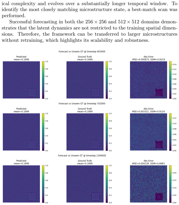
[Section 2.3.2, Figure 7] The 512×512 experiment was evaluated using a 'best-match scan' in which the prediction is compared with multiple future ground-truth states and the most closely matching state is selected. This is not a fixed-horizon prediction test: it can conceal temporal drift, because a model that produces the correct morphology at the wrong time can be scored as accurate. No quantitative error values are reported for the 512×512 case. Since the Abstract explicitly claims successful transfer to 512×512 domains, please provide fixed-horizon metrics (e.g., MSE/SSIM at specified future timesteps) and clarify how temporal alignment was handled.
[Abstract, Section 1, Section 2.3, Section 4.8.1, Discussion] The training-domain size is stated inconsistently: the Abstract, Section 4.8.1, and the Discussion say 100×100, while Section 1 and Section 2.3 say 128×128. The encoder description (100×100×5 → 80×80×128, 6,400 graph nodes) is consistent with 100×100 but not with 128×128. This inconsistency is not merely typographical: it affects the meaning of the claim that the model was 'trained only on 100×100' and the design of the patch-based transfer strategy. Please state the actual training domain size consistently throughout and verify all downstream numbers against it.
[Section 2.1, Sections 4.8.2 and 4.8.4] The headline validation numbers (MSE=8.057e-06, SSIM=0.9993, BCE=2.460e-10, conservation loss=4.497e-16) are the training objectives themselves, evaluated on an in-distribution held-out set. Reporting a conservation term that the loss explicitly enforces as an achieved physical constraint is circular. The manuscript should report quantities that are not directly penalized during training, such as error growth as a function of forecast horizon, conservation of total composition from the predicted fields, and comparison with a simple reference (e.g., persistence or a linear extrapolation). It would also help to state explicitly whether the 3,000,000-timestep forecasts are generated autoregressively step-by-step or in chunks.
[Sections 2.2, 2.4, Table 1] The zero-shot generalization experiments for unseen precipitate count, morphology, and composition report only qualitative visual descriptions and no quantitative error metrics. For the composition variations, Table 1 truncates the evaluation at 327,000 timesteps because 'forecasting fidelity beyond this point decreases more noticeably,' yet the Abstract claims horizons up to 3,000,000 timesteps without qualification. The claim that unseen compositions are forecast 'accurately' is not supported by quantitative evidence. Please provide error-vs-horizon curves and, if the longer composition runs degrade, soften the Abstract claim or report the degradation explicitly.

minor comments (5)

[Section 4.6.1, Eq. (18)] The Allen-Cahn equation for ϕ_BCC appears to contain a duplicated term: '∂fint/∂ϕ_BCC' is written twice, where the second term should presumably be the chemical contribution ∂fchem,bulk/∂ϕ_BCC.
[Section 4.8.1] The dataset description says '1,000 microstructure snapshots' with an (80/10/10) split, but 800+100+101 = 1,001. Please correct the counts. Also 'performed on the The dataset' is a grammatical error.
[References] References are given as raw URLs, many incomplete; several lack author/title/journal details. They should be converted to a standard citation format. [2], [3], [5], [7] and others are not fully descriptive.
[Section 4.2.1] The text refers to 'BCC xx phase'; this is likely a typo for a specific phase name (e.g., BCC_A2 or disordered BCC). Please clarify.
[Figures generally] The figures show qualitative snapshots, but none include quantitative error maps or full time sequences. Adding error-versus-time plots and scale bars would greatly help the reader assess the claimed accuracy.

Circularity Check

1 steps flagged · score 3.0 of 10

Validation metrics are the training objectives; core zero-shot tests remain independent.

fitted input called prediction [Section 2.1 (best epoch metrics) and Section 4.8.2/4.8.4 (composite loss)]
"For model training, a composite loss function is implemented consisting of concentration reconstruction error, structural similarity preservation, phase-field reconstruction loss, and elemental conservation penalties. ... The model’s best performing epoch is 94 with a mean physical-space MSE of 8.057e−06, a mean SSIM of 0.9993, a phase-field BCE of 2.460e−10, and a conservation loss of 4.497e−16 on the held-out validation set."

The reported 'prediction accuracy' metrics are the terms the network was explicitly optimized to minimize: MSE, SSIM, BCE, and conservation are all listed as components of the composite loss. In particular, Methods states that 'conservation constraints are enforced exclusively on the concentration branch' and that conservation is applied by 'enforcing an agreement between the predicted and the ground truth mean compositions.' A near-zero conservation loss is therefore a measure of how well the optimizer satisfied its own enforced penalty, not an independent physical prediction. The held-out split gives some generalization content to MSE/SSIM/BCE, but the conservation value and the corresponding claim that the model 'preserves the conservation constraints learned during training' are tautol

full rationale

The core derivation is data-driven rather than circular: the GCN–LSTM is trained on latent sequences produced from phase-field simulations and then evaluated on held-out and genuinely unseen configurations. The main tautology is that Section 2.1 headlines validation metrics that Section 4.8 defines as the training loss itself — MSE, SSIM, BCE, and conservation penalties. This is especially clear for the conservation loss of 4.497e−16, since conservation is enforced as a loss term, so reporting it as a validation achievement is circular. However, this does not collapse the paper's central claim: the zero-shot tests for unseen precipitate count, size, position, 256×256 transfer, and composition offsets are independent of the fit, and the paper candidly reports known limitations such as initial 256×256 failure ('initial attempts on unseen 256×256 failed due to blurry predictions') and reduced fidelity at larger composition offsets ('forecasting fidelity beyond this point decreases more noticeably'). The 512×512 best-match scan and the absence of reported 512×512 errors are genuine evaluation weaknesses, but they are not circularity in the derivation chain. The self-citation to the authors' prior binary-alloy framework [10] is contextual and not load-bearing for the present validation. The internal inconsistency between 100×100 and 128×128 domain descriptions is an error, not circularity. Overall, there is partial tautological reporting of optimized loss terms, but the central forecasting and generalization results retain independent content, so the circularity score is low-moderate.

Assumptions & free parameters 7 free parameters · 4 assumptions · 0 invented entities

The surrogate's ground truth is the authors' own KKS phase-field code, parameterized inside this paper: tensor-model ranks, mobility, interface parameters, and ad hoc spinodal coefficients are chosen by hand (Sections 4.4-4.6), and the 'unseen' compositions are generated by that same code. Nothing is validated against experiments or an external solver, so every claim in the paper inherits the validity of this ground-truth generator. No new physical entities are introduced; the latent graph nodes and latent vectors are computational constructs without independent physical status.

free parameters (7)

Tensor-model ranks for Gibbs-energy fit (BCC/FCC) = R=10 (BCC), R=6 (FCC)
Chosen by hand 'following the method of [13]' (Section 4.4); the fitted Gibbs energy surface defines all ground-truth diffusion potentials.
Spinodal chemical-potential scaling W_spin = 0.001 x G''
Ad hoc 'to mimic the uphill driving force for diffusion in the spinodal region' (Section 4.6.2); directly shapes the ground-truth spinodal morphology the model learns.
Gradient-energy coefficient epsilon (Phi term) = 0.1 x G''
Ad hoc coefficient multiplying the concentration-gradient energy (Section 4.6.2); sets the gradient-penalty scale in the Cahn-Hilliard equation.
Interface and mobility parameters (kappa, gamma, m, L, M_bulk) = kappa=1e-12, gamma=1.5, m=1e6, L=1.1922e-4, M_bulk=1e-19
Hand-set phase-field parameters (Sections 4.5-4.6) determining interfacial energy, thickness, and kinetics; they set the timescale on which '3,000,000 timesteps' has physical meaning.
Two-phase and spinodal region thresholds = two-phase: 0<f_BCC_B2#1<1; spinodal: 0.1<f_BCC_B2#1<0.9
Hand-chosen boundaries (Section 4.4) controlling where Phi=1 and the W_spin term applies; they decide the map from composition fields to the modified evolution equations.
Snapshot cadence and input sequence length = every 3,000 steps; sequences of length 3
Data-formatting choices (Section 4.8.1) that define the discrete forecasting problem; the adaptive timestep means physical time between snapshots is not constant and is not specified.
AE-GCN-LSTM hyperparameters = latent 80x80x128, hidden 256, 4 GCN layers, lr 2e-4, wd 1e-5
Hand-chosen architecture and training settings (Sections 4.8.2-4.8.4); standard ML choices, but the paper's accuracy claims are specific to them.

assumptions (4)

standard math KKS equal-diffusion-potential construction: phase compositions are computed from equal chemical potentials in the two phases plus local mass conservation (Section 4.2.2).
Standard phase-field formalism (Kim-Kim-Suzuki, ref [11]); the surrogate inherits the thermodynamics of this construction.
domain assumption CALPHAD Gibbs energies for BCC/FCC phases from Thermo-Calc database TCHEA7 at T=1300 K, approximated by a fitted rank-10/rank-6 tensor model (Section 4.4).
Ground-truth thermodynamics are taken from a database and a polynomial fit of it; errors here propagate into the training data and every accuracy metric.
domain assumption The authors' own phase-field equations (Allen-Cahn for order parameters, Cahn-Hilliard with an ad hoc spinodal term in the chemical potential) generate the true microstructure evolution (Sections 4.6.1-4.6.2).
The surrogate is trained and validated exclusively against this code; no experimental or third-party benchmark appears anywhere in the paper.
ad hoc to paper Transferability: latent dynamics learned on single-composition, single-precipitate 100x100/128x128 data are local in latent space and valid across precipitate counts, domain sizes, and nearby compositions (Sections 2.3-2.4).
The patch-based stitching and zero-shot composition tests require this; the paper's own failure modes (blurry 256x256 forecasts, fidelity drop past 327,000 steps) bound its validity.

how reviews work

0 comments

Cite this review

Pith. "Pith review of Deep Learning for Accelerated Long-Horizon Forecasting of Multicomponent Multiphase Microstructure Evolution in High-Entropy Alloys." pith.science (2026). https://pith.science/paper/25XT65BD

@misc{pith2026260727820,
  author       = {Pith},
  title        = {Pith review of: Deep Learning for Accelerated Long-Horizon Forecasting of Multicomponent Multiphase Microstructure Evolution in High-Entropy Alloys},
  year         = {2026},
  howpublished = {\url{https://pith.science/paper/25XT65BD}},
  note         = {Machine review of arXiv:2607.27820}
}

read the original abstract

Phase-field modeling provides a powerful approach for predicting microstructure evolution but becomes computationally prohibitive for multicomponent and multiphase systems over large spatial and temporal scales. This work presents an AE-GCN-LSTM surrogate framework for long-horizon forecasting of microstructure evolution in the multicomponent AlCrFeNi high-entropy alloy system containing coexisting BCC and FCC phases. A multi-head autoencoder compresses the four elemental concentration fields and phase-field order parameter into latent representations, which are formulated as graphs for learning their spatial and temporal evolution. The framework accurately forecasts microstructure evolution over horizons extending to 3,000,000 simulation timesteps. Its robustness is systematically evaluated under previously unseen conditions without retraining, fine-tuning, or parameter adaptation. These evaluations include variations in FCC precipitate size and initial position, microstructures containing one, two, and five FCC precipitates, and complex phase interactions involving precipitate merging and splitting. Although trained only on 100 x 100 computational domains containing a single nominal alloy composition, the framework is successfully transferred to larger 256 x 256 and 512 x 512 systems and to previously unseen AlCrFeNi compositions. Across the evaluated configurations, the model preserves the dominant phase morphology and compositional evolution while providing computational speedups ranging from approximately 7200 to 62300 relative to conventional phase-field simulations. These results demonstrate that latent graph-based AE-GCN-LSTM forecasting provides a scalable and computationally efficient surrogate for long-horizon simulation of multicomponent, multiphase microstructures and offers a promising foundation for high-throughput alloy design.

Figures

Figures reproduced from arXiv: 2607.27820 by the authors.

**Figure 2.** Single small FCC forecasting up to 1,644,000 timesteps. 2.2.2 Single Large FCC Precipitate Configuration The second study examined a microstructure containing a significantly larger FCC precipitate Relative to the training configurations. This dataset introduces a considerably different phase morphology and precipitate volume fraction. This configuration evaluates whether the latent-space forecasting framework can a… view at source ↗

**Figure 3.** Single large FCC forecasting up to 3,000,000 timesteps. 2.2.3 Dual FCC Precipitate Configuration The third generalization study considered a microstructure containing two FCC precipitates. This configuration introduces additional phase interfaces and more complex spatial interactions compared to the single-precipitate cases. Since the model was not exposed to this morphology during training, this dataset provides a … view at source ↗

Figures from the paper (8 more)

**Figure 4.** Figure 4: Dual FCC FCC forecasting up to 3,000,000 timesteps. 2.2.4 Five FCC Precipitate Configuration The final study considered an unseen microstructure containing five FCC precipitates distributed throughout the computational domain. Compared with previous configurations, th…

**Figure 5.** Figure 5: Five FCC forecasting up to 3,000,000 timesteps. 2.3 Generalization to Unseen Spatial Resolutions In addition to morphological variations, the scalability of the proposed framework was evaluated on microstructures with spatial resolutions that were not encountered duri…

**Figure 6.** Figure 6: Forecasting of 256 × 256 up to 3,000,000 timesteps. 2.3.2 Generalization to a 512 × 512 Domain The same patch-based forecasting strategy from the previous study was further applied to an unseen 512 × 512 microstructure. This facilitates evaluating whether the learned …

**Figure 7.** Figure 7: Forecasting of 512 × 512 up to 1,290,000 timesteps. 2.4 Generalization to Unseen Alloy Compositions This section assesses whether a model trained on a single nominal composition can accurately predict the evolution of the microstructure under an unseen alloy compositi…

**Figure 8.** Figure 8: Forecasting under unseen ±1% composition variation. 2.4.2 ±0.02 Composition Variation For the ±0.02 variations, the resulting forecasts preserved the dominant precipitate morphology and the overall compositional balance. However, relative to the ±0.01 perturbation, th…

**Figure 9.** Figure 9: Forecasting under unseen ±2% composition variation. 2.5 Runtime Comparison [PITH_FULL_IMAGE:figures/full_fig_p013_9.png]

**Figure 10.** Figure 10: Encoding of input microstructures into a latent representation. Re [PITH_FULL_IMAGE:figures/full_fig_p021_10.png]

**Figure 11.** Figure 11: Graph representation of the encoded latent microstructure. Nodes [PITH_FULL_IMAGE:figures/full_fig_p022_11.png]

Discussion (0). Continue with ORCID to comment.

Reference graph

Works this paper leans on

21 extracted references · 4 canonical work pages

[1]

https://www.sciencedirect.com/science/article/pii/S0364591607000880
[2]

https://link.springer.com/article/10.1186/s40323-024-00280-4

work page doi:10.1186/s40323-024-00280-4
[3]

https://www.sciencedirect.com/science/article/pii/S2238785426003157?via
[4]

https://www.sciencedirect.com/science/article/abs/pii/S1359645425008894?via
[5]

https://pubs.acs.org/aaemdr/article-abstract/doi/10.1021/acsaenm.6c00545/5204700/Bridging- Phase-Field-Model-and-Deep-Learning-for?redirectedFrom=fulltext

work page doi:10.1021/acsaenm.6c00545/5204700/bridging-
[6]

https://link.springer.com/article/10.1007/s00366-025-02117-z

work page doi:10.1007/s00366-025-02117-z
[7]

https://www.nature.com/articles/s41524-024-01324-4
[8]

https://www.sciencedirect.com/science/article/abs/pii/S0927025624007390

Show all 21 references

[9]

https://www.sciencedirect.com/science/article/abs/pii/S0927025622004645
[10]

https://www.nature.com/articles/s41524-026-01999-x
[11]

http://link.aps.org/doi/10.1103/PhysRevE.60.7186,

doi
[12]

https://www.sciencedirect.com/science/article/abs/pii/S1359645410007019,
[13]

https://www.nature.com/articles/s41524-019-0268-y,
[14]

https://www.science.org/doi/10.1126/science.1127647 23

doi
[15]

(2023), Autoencoders (Machine Learning with Applications review) https://link.springer.com/chapter/10.1007/978-3-031-24628-9 16

Bank et al. (2023), Autoencoders (Machine Learning with Applications review) https://link.springer.com/chapter/10.1007/978-3-031-24628-9 16

2023 doi
[16]

https://ieeexplore.ieee.org/document/1284395
[17]

https://www.semanticscholar.org/paper/Semi- Supervised-Classification-with-Graph-Networks-Kipf- Welling/36eff562f65125511b5dfab68ce7f7a943c27478
[18]

https://dl.acm.org/doi/10.1162/neco.1997.9.8.1735

1997 doi
[19]

https://dl.acm.org/doi/10.5555/3045118.3045167
[20]

https://www.semanticscholar.org/paper/Layer-Normalization-Ba- Kiros/97fb4e3d45bb098e27e0071448b6152217bd35a5
[21]

https://dl.acm.org/doi/abs/10.5555/2627435.2670313 24

Pith tools

Reviewed August 1, 2026 · model on record in the stance chip above.

[1] [1]

https://www.sciencedirect.com/science/article/pii/S0364591607000880

[2] [2]

https://link.springer.com/article/10.1186/s40323-024-00280-4

work page doi:10.1186/s40323-024-00280-4

[3] [3]

https://www.sciencedirect.com/science/article/pii/S2238785426003157?via

[4] [4]

https://www.sciencedirect.com/science/article/abs/pii/S1359645425008894?via

[5] [5]

https://pubs.acs.org/aaemdr/article-abstract/doi/10.1021/acsaenm.6c00545/5204700/Bridging- Phase-Field-Model-and-Deep-Learning-for?redirectedFrom=fulltext

work page doi:10.1021/acsaenm.6c00545/5204700/bridging-

[6] [6]

https://link.springer.com/article/10.1007/s00366-025-02117-z

work page doi:10.1007/s00366-025-02117-z

[7] [7]

https://www.nature.com/articles/s41524-024-01324-4

[8] [8]

https://www.sciencedirect.com/science/article/abs/pii/S0927025624007390