Quantum Backreaction in Effective Brans-Dicke Bianchi I Cosmology
Pith reviewed 2026-05-16 13:45 UTC · model grok-4.3
The pith
Cross-correlation terms between quantum fluctuations are required to prevent divergences and maintain physical consistency in Brans-Dicke Bianchi I cosmology.
A machine-rendered reading of the paper's core claim, the machinery that carries it, and where it could break.
Core claim
In the effective Hamiltonian formalism for quantum Brans-Dicke Bianchi I cosmology, cross-correlation terms between different degrees of freedom are essential; neglecting them causes spurious divergences, uncertainty principle violations, and unphysical behavior, whereas including them smooths bounces for w less than -3/2, accelerates de Sitter approach for w equals -3/2, keeps energy density finite, and produces damped oscillations interpreted as quantum remnants.
What carries the argument
Effective Hamiltonian truncation retaining expectation values, quantum dispersions, and cross-correlation terms between gravitational and scalar field degrees of freedom.
If this is right
- For w less than -3/2, quantum backreaction smooths the bounce, suppresses shear anisotropy, and keeps the energy density peak finite and well-behaved.
- For the conformally invariant case w equals -3/2, quantum corrections accelerate the approach to de Sitter expansion while enhancing shear anisotropy.
- Small-amplitude damped oscillations appear shortly after the bounce and encode Planck-scale correlation information.
- The effective energy density remains finite across both regimes when cross-correlations are retained.
Where Pith is reading between the lines
- Similar correlation terms may be required for consistency in other effective quantum cosmologies, including loop quantum gravity or string-inspired models.
- Primordial observables such as gravitational wave spectra could carry imprints of these quantum remnant oscillations.
- This suggests that inter-field quantum information influences the transition from Planck-scale to classical cosmology in anisotropic settings.
Load-bearing premise
The truncation to expectation values, dispersions, and cross-correlations is sufficient to capture leading quantum backreaction without higher-order moments or full quantum gravity corrections.
What would settle it
A full quantum simulation of the system that shows uncertainty relations violated or observables diverging when cross-correlations are omitted would confirm their necessity.
Figures


read the original abstract
We investigate the effective quantum evolution of the Bianchi type I cosmological model within the Brans-Dicke framework, using an effective Hamiltonian approach including expectation values, quantum dispersions, and cross-correlation terms between different degrees of freedom. We show that cross-correlation terms are essential for a physically consistent effective dynamics: neglecting them leads to spurious divergences, violation of the Heisenberg uncertainty relations, and unphysical behavior. For w < -3/2, where bouncing solutions exist already classically, quantum backreaction smooths the bounce, suppresses shear anisotropy, and the energy density peak is slightly enhanced and remains well-behaved, in contrast to the unphysical divergences that arise when cross-correlations are neglected. For the conformally invariant case w = -3/2, quantum corrections accelerate the approach to de Sitter expansion while enhancing shear anisotropy. When correlations are included, small-amplitude damped oscillations appear shortly after the bounce, which we interpret as quantum remnant effects encoding Planck scale correlation information between gravitational and scalar field degrees of freedom. The effective energy density remains finite for both regimes. Our results demonstrate that cross-correlations carry crucial quantum information influencing cosmological dynamics, with implications for quantum gravity phenomenology, inflationary model building, and primordial observational signatures.
Editorial analysis
A structured set of objections, weighed in public.
Referee Report
Summary. The paper investigates the effective quantum evolution of the Bianchi type I cosmological model in the Brans-Dicke framework via a second-moment truncation of the effective Hamiltonian that retains expectation values, dispersions, and cross-correlations between gravitational and scalar degrees of freedom. It claims that cross-correlation terms are required for physical consistency: their omission produces spurious divergences, Heisenberg uncertainty violations, and unphysical behavior, while their inclusion yields a smoothed bounce with suppressed shear for w < -3/2 and accelerated de Sitter expansion with small damped oscillations for the conformally invariant case w = -3/2, keeping the effective energy density finite in both regimes.
Significance. If the second-moment truncation remains valid, the results would establish that quantum cross-correlations carry essential information for consistent effective dynamics in anisotropic quantum cosmology, with potential implications for bounce phenomenology, shear suppression, and primordial signatures. The explicit demonstration that neglecting correlations violates basic quantum principles strengthens the case for retaining them in effective quantum gravity models.
major comments (2)
- [Abstract] Abstract and effective Hamiltonian truncation: the central claim that cross-correlations remove divergences and restore uncertainty-principle compliance rests on an unshown derivation; no explicit equations, numerical plots, or error estimates demonstrating the cancellation are visible, leaving the load-bearing step unsupported.
- [Effective dynamics section] The second-moment truncation implicitly assumes higher-order moments remain perturbatively small near the bounce, yet no consistency check or bound on third- and higher-order moments is provided for either w < -3/2 or w = -3/2; if these moments grow, they could feed back into the reported smoothing and oscillation results.
minor comments (2)
- [Introduction] Notation for the Brans-Dicke parameter w and the cross-correlation functions should be defined explicitly at first use to improve readability.
- [Results] Figure captions for the energy-density and shear plots should include the specific values of w and initial conditions used.
Simulated Author's Rebuttal
We thank the referee for the careful reading and constructive comments on our manuscript. We address the major concerns point by point below, indicating the revisions we will implement to strengthen the presentation and support for our claims.
read point-by-point responses
-
Referee: [Abstract] Abstract and effective Hamiltonian truncation: the central claim that cross-correlations remove divergences and restore uncertainty-principle compliance rests on an unshown derivation; no explicit equations, numerical plots, or error estimates demonstrating the cancellation are visible, leaving the load-bearing step unsupported.
Authors: We agree that the central claim requires more explicit support. Although the effective equations including cross-correlations are derived in Section 3, we will revise the manuscript to add the explicit expressions for the relevant Hamiltonian terms with and without correlations, include additional numerical plots showing the time evolution of key quantities (demonstrating divergence cancellation and uncertainty-principle compliance), and report numerical error estimates from our integration scheme. revision: yes
-
Referee: [Effective dynamics section] The second-moment truncation implicitly assumes higher-order moments remain perturbatively small near the bounce, yet no consistency check or bound on third- and higher-order moments is provided for either w < -3/2 or w = -3/2; if these moments grow, they could feed back into the reported smoothing and oscillation results.
Authors: The second-moment truncation is a standard approximation in effective quantum cosmology. We acknowledge that the current manuscript lacks an explicit consistency check or bound on higher moments. In the revision we will add a discussion in the effective dynamics section on the perturbative validity of the truncation near the bounce, based on the observed numerical behavior. A full quantitative bound on the moment hierarchy lies beyond the scope of this work. revision: partial
Circularity Check
No significant circularity; effective truncation shown by explicit comparison
full rationale
The paper derives the effective dynamics from a truncated moment hierarchy (expectation values + dispersions + cross-correlations) and demonstrates necessity of the cross terms by direct substitution into the equations of motion, producing divergences and uncertainty violations when they are dropped. No parameter is fitted to the target observables and then relabeled as a prediction; no load-bearing uniqueness theorem or ansatz is imported via self-citation; the central result follows from the algebra of the truncated Poisson brackets rather than from redefinition of the inputs. The derivation remains self-contained against the stated truncation assumption.
Axiom & Free-Parameter Ledger
free parameters (1)
- Brans-Dicke parameter w
axioms (2)
- domain assumption The effective dynamics can be closed at the level of expectation values plus second moments.
- standard math Heisenberg uncertainty relations must be satisfied by the effective variables.
Lean theorems connected to this paper
-
IndisputableMonolith/Cost/FunctionalEquation.leanwashburn_uniqueness_aczel unclear?
unclearRelation between the paper passage and the cited Recognition theorem.
Heff = H_cl + H^(2)(Δ(q^a p^b)) + O(ℏ^{3/2}); truncation at second order in moments with cross-correlations Δ(c_i p_j) for i≠j
-
IndisputableMonolith/Foundation/RealityFromDistinction.leanreality_from_one_distinction unclear?
unclearRelation between the paper passage and the cited Recognition theorem.
No reference to recognition cost, φ, 8-tick clock, or derivation from ∃x y (x≠y)
What do these tags mean?
- matches
- The paper's claim is directly supported by a theorem in the formal canon.
- supports
- The theorem supports part of the paper's argument, but the paper may add assumptions or extra steps.
- extends
- The paper goes beyond the formal theorem; the theorem is a base layer rather than the whole result.
- uses
- The paper appears to rely on the theorem as machinery.
- contradicts
- The paper's claim conflicts with a theorem or certificate in the canon.
- unclear
- Pith found a possible connection, but the passage is too broad, indirect, or ambiguous to say the theorem truly supports the claim.
Forward citations
Cited by 1 Pith paper
-
Quantum corrections to cosmic perturbations for a bouncing background
In an LQC bouncing cosmology, second-order quantum moments yield a Planck-suppressed scale-dependent correction δP_R ∝ (k ℓ_Pl)^6 to the curvature power spectrum together with post-bounce damping from gravitational moments.
Reference graph
Works this paper leans on
-
[1]
Bianchi I Geometry and Canonical Variables The Bianchi type I model describes spatially homoge- neous, anisotropic, and spatially flat cosmologies. The metric takes the diagonal form ds2 =−N 2dt2 +a 2 1(t)dx2 1 +a 2 2(t)dx2 2 +a 2 3(t)dx2 3,(2) whereN(t) is the lapse function anda i(t) are directional scale factors. Spatial homogeneity allows reduction to...
-
[2]
We work in units where 16πG= 1 and setγ= 1 for simplicity
Brans-Dicke Action and Hamiltonian Constraint The Brans-Dicke action is [7, 10] SBD = 1 16π Z d4x√−g ϕR− ω ϕ gµν∂µϕ∂νϕ ,(8) whereϕis the Brans-Dicke scalar (related to the gravita- tional constant byG eff = 1/ϕ) andωis the dimensionless coupling constant. We work in units where 16πG= 1 and setγ= 1 for simplicity. The Barbero–Immirzi parameter γcan take an...
-
[3]
Physical Energy Densities To identify the physical energy density, we compare the BD Hamiltonian constraints with the standard GR Friedmann structure. In the isotropic limit where allc i = Candp i =P, the GR Hamiltonian constraint is [41] H=− 3 8πGγ2 C2p |P|+H matter ≈0,(13) 4 where the vanishing of the constraint gives the Friedmann equationH 2 = (8πG/3)...
-
[4]
Equations of Motion Hamilton’s equations ˙f={f,H BD}with the con- straint (9) yield (settingN=γ= 1): ˙c1 = 1 ϕ√p h −c1(c2p2 +c 3p3 −2ζT) + S−ζT 2 2p1 i , ˙c2 = 1 ϕ√p h −c2(c1p1 +c 3p3 −2ζT) + S−ζT 2 2p2 i , ˙c3 = 1 ϕ√p h −c3(c1p1 +c 2p2 −2ζT) + S−ζT 2 2p3 i , ˙p1 = √p ϕ c2p3 +c 3p2 − 2p1ζT p , ˙p2 = √p ϕ c1p3 +c 3p1 − 2p2ζT p , ˙p3 = √p ϕ c1p2 +c 2p1 − 2p...
-
[5]
Bouncing Solutions and Initial Conditions Forω <−3/2, the parameterζ <0, and the term −ζT 2 >0 in the Hamiltonian constraint (9) can dom- FIG. 1. Classical evolution of directional scale factorsa i(t) for Brans-Dicke Bianchi I withω=−5. All three directions exhibit smooth bounces, with anisotropic structure evident in different bounce amplitudes. Initial ...
-
[6]
Numerical Results Figure 1 shows the evolution of scale factorsa i(t) ob- tained by numerical integration of Eqs. (16). All three di- rectional scale factors exhibit smooth bounces neart≈0, with minimum valuesa min i ∼(0.8-1.1) depending on di- rection. The anisotropy is evident: different directions have different bounce times and minimum scales. Figure ...
-
[7]
De Sitter Asymptotics An interesting feature of theω= -3/2 case is its asymp- totic de Sitter behavior [18]. From Eq. (18), one can show that ast→ ±∞, eachH i approaches a constant value Hi →H ∞, implying exponential expansion (or contrac- tion)a i ∼e H∞t. This is related to conformal invariance: the theory admits solutions asymptotically approaching de S...
-
[8]
Numerical Results We evolve Eqs. (18) with initial conditions c1(0) = 1.1, p 1(0) = 1.0, c2(0) = 1.2, p 2(0) = 2.0, c3(0) = 1.3, p 3(0) = 3.0, ϕ(0) = 10, p ϕ(0) = 1.0,(21) andλ= 1. While physical observables areλ-independent when ex- pressed in terms of the relationalϕ, we present numerical results as functions of coordinate timetwith the gauge choiceλ= 1...
-
[9]
Quantum Moments and Extended Phase Space Consider a quantum system with canonical variables (ˆqi,ˆpi) satisfying [ˆqi,ˆpj] =iℏδ ij. We define expectation values ⟨ˆqi⟩ ≡q i,⟨ˆp i⟩ ≡p i,(22) and quantum moments (using Weyl ordering for sym- metrization): ∆(qa i pb j)≡ ⟨(ˆqi −q i)a(ˆpj −p j)b⟩Weyl.(23) Witha+b= 2. The correlations and moments: ∆(q2 i ) =⟨(ˆq...
-
[10]
Effective Hamiltonian and Equations of Motion The effective Hamiltonian is defined as the expectation value of the quantum Hamiltonian operator: Heff =⟨ ˆH⟩.(26) Expanding in powers of quantum moments: Heff =H cl(q, p) + ∞X n=2 H(n)(∆(qapb)),(27) whereH cl is the classical Hamiltonian andH (n) contains contributions from moments of ordern. Formally, this ...
-
[11]
Since mo- ments scale as ∆(qapb)∼ℏ (a+b)/2, the expansion is effec- tively in powers ofℏ
Truncation and Hierarchy The expansion (27) is, in general, infinite, so, for prac- tical calculations, we truncate at finite order. Since mo- ments scale as ∆(qapb)∼ℏ (a+b)/2, the expansion is effec- tively in powers ofℏ. Truncation at second order yields the following semiclassical approximation: Heff ≈H cl +H (2)(∆(q2),∆(p 2),∆(qp), . . .) +O(ℏ 3/2). (...
-
[12]
Phase Space and Quantum Variables Our system hask= 4 canonical pairs: (c i, pi) fori= 1,2,3 and (ϕ, p ϕ). At second order, the relevant quantum variables are: •Expectation values (8):c 1, c2, c3, p1, p2, p3, ϕ, pϕ •Diagonal moments (8): ∆(c 2 i ),∆(p 2 i ) fori= 1,2,3; ∆(ϕ2),∆(p 2 ϕ) •Covariances (4): ∆(c ipi) fori= 1,2,3; ∆(ϕp ϕ) •Cross-correlations (28)...
-
[13]
Second-Order Effective Hamiltonian:ω <−3/2. Applying the Taylor expansion (28) to the classical Hamiltonian (9) and computing derivatives up to second order, we obtain (settingN=γ= 1): H(ω) eff =HBD + 1√p " 3X i=1 p2 i ζ ϕ ∆(c2 i ) + 1 2ϕ Ai∆(p2 i ) + ζϕ ϕ ∆(p2 ϕ) + 1 2ϕ2 B∆(ϕ2) + 2ζ∆(ϕpϕ) + 3X i=1 Ci∆(cipi) + 2piζ√p ∆(cipϕ) +D i∆(ciϕ) + X i<j (Eij∆(cicj)...
-
[14]
Second-Order Effective Hamiltonian:ω=−3/2. For the conformally invariant case, we expand (11): H(c) eff =H c BD −λ∆(ϕp ϕ) + 1 ϕ2√p " 3X i=1 Ac i∆(p2 i ) +ϕA c i∆(cipi) − S ϕ ∆(ϕ2) + 3X i=1 (Dc i ∆(ciϕ) +J c i ∆(piϕ)) + X i<j E c ij∆(cicj) +F c ij∆(cipj) +G c ij∆(pipj) −ϕ 3X i=1 ∆(cicj)|j̸=i # .(34) 9 C. Validity and Limitations of the Effective Approach
-
[15]
Semiclassicality Conditions For the second-order truncation to be reliable, quan- tum fluctuations must remain small compared to expec- tation values. Define dimensionless ratios: rci ≡ p ∆(c2 i ) |ci| , r pi ≡ p ∆(p2 i ) |pi| .(35) Semiclassicality requiresr ci , rpi to be small far from the bounce. We verify this condition a posteriori in our nu- merica...
-
[16]
It is expected to break down when:
Quantum Gravity Scale and Breakdown The effective approach describes quantum corrections to classical dynamics but does not capture full quantum gravity effects such as spacetime superpositions or topol- ogy change. It is expected to break down when:
-
[17]
Curvature approaches Planck scale:R∼ℓ −2 Pl
-
[18]
Volume approaches Planck scale:V∼ℓ 3 Pl
-
[19]
For our Brans-Dicke model, the effective gravitational constant isG eff = 1/ϕ
Quantum fluctuations become of order unity: rci , rpi ∼1. For our Brans-Dicke model, the effective gravitational constant isG eff = 1/ϕ. The Planck length is therefore ℓPl ∼ϕ −1/2. Near the bounce, withϕ(0) = 10 (in our units), we haveℓ Pl ∼0.3. The minimum scale factor valuesa min i ∼1 correspond to volumesV∼1, which is∼ 101.5 times the Planck volume. Th...
-
[20]
Loop quantum cos- mology for Brans-Dicke Bianchi I has been studied in Refs
Comparison with Loop Quantum Cosmology A natural question is how our effective approach com- pares to full loop quantization. Loop quantum cos- mology for Brans-Dicke Bianchi I has been studied in Refs. [38, 44]. Among the most important differences we can mention the following •LQC quantizes the connection via holonomies, in- troducing a fundamental disc...
-
[21]
Critical Importance of Cross-Correlations We begin by demonstrating that cross-correlation terms are essential for obtaining physically consistent ef- fective dynamics. Figure 9 compares the evolution of the mean scale factora(t) with (bottom) and without (top) cross- correlation terms. When cross-correlations are neglected (setting all ∆(c ipj)|i̸=j = 0,...
-
[22]
Evolution of Mean Scale factor and Quantum Smoothing Once the cross-correlation terms are included, the ef- fective evolution of the mean scale factor shows a less pronounced bounce compared to the classical trajectory FIG. 9. Effective evolution ofa(t) forω=−5 with and without cross-correlation terms included, shown for different quantum state widthsσ χ....
-
[23]
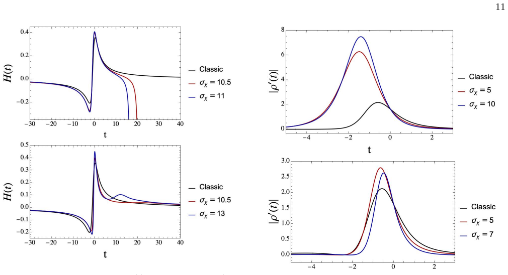
Hubble Parameters and Post-Bounce Oscillations Figure 10 shows the mean directional Hubble param- eterH(t) for variousσ χ. The classical evolution transi- tions smoothly from negative (contraction) through zero (bounce) to positive (expansion). As in figure (9), the pathologies in the effective evolution disappear once the cross-correlation terms are incl...
-
[24]
(14) with quantum corrections, is shown in Fig
Energy Density Evolution The effective energy density, computed from Eq. (14) with quantum corrections, is shown in Fig. 11. Key features displayed are: •Peak enhancement:With cross-correlations in- cluded, the peak valueρ ′ max is slightly increased compared to the classical case. The energy density remains sharply localized near the bounce, qual- itativ...
-
[25]
Shear Evolution and Anisotropy Suppression Figure 12 shows the shear Σ 2(t) evolution. In con- trast to the classical case where shear peaks sharply at the bounce, the effective evolution with cross-correlations shows an anisotropy suppression. We can also notice post-bounce oscillations in the shear, consistent with Hubble parameter oscillations. This an...
-
[26]
Figure 13 shows the evolution of position and momen- tum dispersions ∆(p 2
Evolution of Quantum Moments To understand the microscopic origin of quantum back- reaction, we examine the evolution of key quantum mo- ments themselves. Figure 13 shows the evolution of position and momen- tum dispersions ∆(p 2
-
[27]
forσ χ = 6. We can observe that near the bounce, ∆(p 2 i ) decreases (momentum squeezing) while ∆(c 2 i ) increases (position spreading). This reflects quantum state deformation due to strong gravitational effects. Figure 14 shows evolution of selected cross- correlations: ∆(c 1p2), ∆(c2p3), and ∆(p 1c3). FIG. 13. Evolution of quantum dispersions forω=−5,...
-
[28]
We can notice that the maximum corrections occur at the bounce:δ max ≈0.42
Quantifying Quantum Corrections To quantify the magnitude of quantum backreaction, we define the relative quantum correction to scale factors: δquantum(t) = |aeff(t)−a cl(t)| acl(t) .(40) Figure 15 showsδ quantum(t) forσ χ = 6. We can notice that the maximum corrections occur at the bounce:δ max ≈0.42. This confirms that quantum effects are strong enough ...
-
[29]
Energy Density and Shear The energy density (Fig. 18) exhibits a slight increase in the peak maximum, similar to theω=−5 case, con- firming this is a generic quantum effect. Shear evolution (Fig. 19) shows a key difference from ω=−5: here, the anisotropy increases withσ χ rather than decreasing. This anisotropy enhancement is puzzling and warrants further...
-
[30]
Constraint Violation Monitoring The Hamiltonian constraint must be satisfied through- out evolution:H eff ≈0. For this we analyze ν(t) = |Heff(t)| maxt′ |Heff(t′)| .(41) This relative normalization is chosen because the con- straint is imposed as an initial conditionH eff(0)≈0 and then monitored for drift; dividing by the maximum value provides a scale-in...
-
[31]
Heisenberg Uncertainty Verification For each degree of freedom, all quantum moments must satisfy the generalized Heisenberg uncertainty relation Ξi(t)≡∆(c 2 i )∆(p2 i )−∆(c ipi)2 − ℏ2 4 ≥0.(42) This is satisfied for bothω=−5 andω=−3/2 models throughout the evolution, confirming the physical consis- tency of our quantum states
-
[32]
Semiclassicality Monitoring We compute the semiclassicality ratiosr pi in (35) throughout evolution. Figure 20 shows these ratios for ω=−5,σ χ = 8, andω=−3/2,σ χ = 2.5 remain small for relatively large quantum states width, justify- ing the second-order truncation. Near the bounce, ratios increase as quantum effects become more significant, but remain in ...
-
[33]
Including all 28 cross-correlation terms yields smooth, con- sistent dynamics
Cross-correlations are essential: Neglecting quan- tum correlations between different degrees of free- dom produces nonphysical pathologies. Including all 28 cross-correlation terms yields smooth, con- sistent dynamics
-
[34]
Quantum smoothing: For bothω=−5 andω= −3/2, quantum effects smooth the bounce, spread- ing it over larger time intervals and preventing col- lapse to arbitrarily small scales
-
[35]
These are quantum rem- nant effects encoding correlation information
Post-bounce oscillations: Damped oscillations ap- pear in Hubble parameters and other observables shortly after the bounce. These are quantum rem- nant effects encoding correlation information
-
[36]
Energy density enhancement: quantum effects cause the energy density to concentrate in a region close to the cosmic bounce similar to the classic evolution, increasing the classical peak
-
[37]
Anisotropy modification: Forω=−5, quantum ef- fects suppress anisotropy.ω=−3/2 they enhance it
-
[38]
De Sitter acceleration (ω=−3/2): Quantum ef- fects cause the system to reach De Sitter expansion phases more rapidly, potentially relevant for infla- tionary dynamics
-
[39]
Semiclassical validity: For small values ofσ χ, semi- classicality ratios remain<1.5, and Heisenberg relations are satisfied, justifying the second-order truncation. V. DISCUSSION, CONCLUSIONS AND OUTLOOK A. Summary of Main Results We have investigated the effective quantum evolution of Bianchi type I cosmological models within Brans-Dicke theory, employi...
-
[40]
Cross-correlations are essential: Our most impor- tant result is the demonstration that quantum cross-correlation terms, coupling different spatial directions and geometry to the scalar field, are ab- solutely necessary for physically consistent effective dynamics. Neglecting these 28 cross-correlation terms (for our model) produces spurious patholo- gies...
-
[41]
Quantum smoothing of bounces: For bothω=−5 andω=−3/2, quantum backreaction smooths classical bounces. The bounce becomes more grad- ual, the minimum scale factor increases withσ χ, and the energy density peak is slightly suppressed relative to the classical value, with the suppression growing withσ χ. The unphysical spike that ap- pears when cross-correla...
-
[42]
Post-bounce oscillatory remnants: Damped oscil- lations appear in Hubble parameters and other observables shortly after the bounce. These are direct manifestations of cross-correlation dynam- ics — quantum remnant effects that classical evo- lution cannot produce. They represent transient quantum memory of correlations developed during the Planck-scale bo...
-
[43]
Anisotropy modification: Quantum effects suppress shear anisotropy forω=−5, potentially contribut- ing to the observed near-isotropy of the universe despite BKL expectations [22, 23]. Forω=−3/2, quantum effects instead enhance anisotropy, a puz- zling result whose origin may lie in the conformal constraint structure (12), the exponential decay of ϕ, or hi...
-
[44]
Accelerated de Sitter approach (ω=−3/2): For the conformally invariant case, quantum correc- tions cause the system to reach asymptotic de Sitter expansion more rapidly than classically. This quan- tum acceleration mechanism may relax fine-tuning requirements on initial conditions for inflation, and connects to the equivalence betweenω=−3/2 16 BD and Pala...
-
[45]
Semiclassical validity confirmed: Throughout our parameter range, semiclassicality ratios remainr < 1.5 and Heisenberg uncertainty relations are satis- fied, validating the second-order truncation. We note that the Gaussian truncation argument is weakest near the bounce whereH eff →0 on- shell, and higher-order correctionsO(ℏ 3/2) may be non-negligible th...
work page 2025
-
[46]
ADM Decomposition of Spacetime The Arnowitt-Deser-Misner (ADM) formulation [48] provides a Hamiltonian description of general relativity by decomposing spacetime into space and time. a. Foliation and Line Element Consider a spacetime manifoldMfoliated by spacelike hypersurfaces Σ t labeled by time coordinatet. The line element takes the form ds2 =−N 2dt2 ...
-
[47]
Ashtekar-Barbero Variables The Ashtekar formulation [49] recasts the gravitational phase space in terms of anSU(2) connection and its con- jugate. 18 a. Densitized Triad and Connection Introduce a spatial triade i a(x) such that qab =δ ijei aej b,(A10) with inverse (co-triad)e a i satisfyinge a i ej a =δ j i ande a i eb i = δb a. Define the densitized tri...
-
[48]
Brans-Dicke Theory in ADM Variables a. ADM Decomposition of BD Action The Brans-Dicke action (8) in ADM form becomes SBD = Z dt Z Σ d3x N√q h ϕ (3)R+K abK ab −K 2 − ω ϕN2 ˙ϕ−N a∂aϕ 2 + ω ϕ qab∂aϕ∂bϕ + 2 N ˙ϕ−N a∂aϕ K i . (A17) b. Canonical Variables for Scalar Field The scalar field has canonical momentum pϕ = δLBD δ ˙ϕ = 2√q N Kϕ− ω ϕ ( ˙ϕ−N a∂aϕ) ,(A18)...
-
[49]
Bianchi I Symmetry Reduction a. Diagonal Metric Ansatz For Bianchi I, the spatial metric is diagonal and homo- geneous: qabdxadxb =a 2 1(t)dx2 1 +a 2 2(t)dx2 2 +a 2 3(t)dx2 3.(A20) Choose a fiducial flat metric ˚q ab with ˚qabdxadxb = dx2 1 +dx 2 2 +dx 2 3. b. Fiducial Cell and Volume Since spacetime is noncompact, integrals over Σ di- verge. We introduce...
-
[50]
Effective Poisson Algebra The quantum moments satisfy a closed Poisson algebra derived from canonical commutation relations [27]. For a single degree of freedom (q, p): {∆(q2),∆(p 2)}= 4∆(qp),(B1a) {∆(q2),∆(qp)}= 2∆(q 2),(B1b) {∆(p2),∆(qp)}=−2∆(p 2),(B1c) {q,∆(q 2)}= 2∆(qp),(B1d) {p,∆(q 2)}= 0,(B1e) {q,∆(p 2)}= 0,(B1f) {p,∆(p 2)}=−2∆(qp),(B1g) {q,∆(qp)}= ...
-
[51]
Equations for Expectation Values:ω̸=−3/2 The evolution of expectation values is given by ˙f= {f, Heff}. For our system: ˙c1 = ∂Heff ∂p1 = ∂HBD ∂p1 + X a,b ∂2HBD ∂p1∂xab ∆(xab),(B3a) ˙c2 = ∂Heff ∂p2 = ∂HBD ∂p2 + X a,b ∂2HBD ∂p2∂xab ∆(xab),(B3b) ˙c3 = ∂Heff ∂p3 = ∂HBD ∂p3 + X a,b ∂2HBD ∂p3∂xab ∆(xab),(B3c) ˙p1 =− ∂Heff ∂c1 =− ∂HBD ∂c1 − X a,b ∂2HBD ∂c1∂xab ...
-
[52]
The full ex- pressions are lengthy; we implement them numerically using Mathematica
+ 2p1ζ√p ∂ ∂p1 ∆(c1pϕ) +· · · , (B4) and similarly for other expectation values. The full ex- pressions are lengthy; we implement them numerically using Mathematica
-
[53]
Equations for Quantum Moments:ω̸=−3/2 For quantum dispersions (diagonal moments), the evo- lution is: 1 2 ˙∆(c2
-
[54]
= ∂2Heff ∂p2 1 ∆(c1p1) + ∂2Heff ∂c1∂p1 ∆(c2 1) + X j̸=1 ∂2Heff ∂p1∂cj ∆(c1cj) + ∂2Heff ∂p1∂pj ∆(c1pj) + ∂2Heff ∂p1∂ϕ ∆(c1ϕ) + ∂2Heff ∂p1∂pϕ ∆(c1pϕ),(B5a) 1 2 ˙∆(p2
-
[55]
For covariances (e.g., ∆(c 1p1)): ˙∆(c1p1) =− ∂2Heff ∂c2 1 ∆(c2
=− ∂2Heff ∂c2 1 ∆(c1p1)− ∂2Heff ∂c1∂p1 ∆(p2 1) − X j̸=1 ∂2Heff ∂c1∂cj ∆(p1cj) + ∂2Heff ∂c1∂pj ∆(p1pj) − ∂2Heff ∂c1∂ϕ ∆(p1ϕ)− ∂2Heff ∂c1∂pϕ ∆(p1pϕ),(B5b) with analogous equations for ∆(c2 2), ∆(p2 2), ∆(c2 3), ∆(p2 3), ∆(ϕ2), ∆(p2 ϕ). For covariances (e.g., ∆(c 1p1)): ˙∆(c1p1) =− ∂2Heff ∂c2 1 ∆(c2
-
[56]
+ ∂2Heff ∂p2 1 ∆(p2 1) − X j̸=1 ∂2Heff ∂c1∂cj ∆(c1cj) + ∂2Heff ∂c1∂pj ∆(c1pj) + X j̸=1 ∂2Heff ∂p1∂cj ∆(p1cj) + ∂2Heff ∂p1∂pj ∆(p1pj) − ∂2Heff ∂c1∂ϕ ∆(c1ϕ) + ∂2Heff ∂p1∂ϕ ∆(p1ϕ) − ∂2Heff ∂c1∂pϕ ∆(c1pϕ) + ∂2Heff ∂p1∂pϕ ∆(p1pϕ). (B6) For cross-correlations (e.g., ∆(c1p2)): ˙∆(c1p2) = ∂2Heff ∂p2 1 ∆(p1p2)− ∂2Heff ∂c2 2 ∆(c1c2) + ∂2Heff ∂c1∂p1 ∆(c1p2)− ∂2Heff ...
- [57]
-
[58]
B. P. Abbott, R. Abbott, T. D. Abbott, M. R. Aber- nathy, F. Acernese, K. Ackley, C. Adams, T. Adams, P. Addesso, R. X. Adhikari,et al., Physical review let- ters116, 061102 (2016)
work page 2016
-
[59]
S. W. Hawking and R. Penrose, Proceedings of the Royal Society of London. A. Mathematical and Physical Sci- ences314, 529 (1970)
work page 1970
-
[60]
V. C. Rubin, W. K. Ford Jr, and N. Thonnard, Astro- physical Journal, Part 1, vol. 238, June 1, 1980, p. 471- 487.238, 471 (1980)
work page 1980
-
[61]
T. M. Abbott, F. B. Abdalla, A. Alarcon, J. Aleksi´ c, S. Allam, S. Allen, A. Amara, J. Annis, J. Asorey, S. Avila,et al., Physical Review D98, 043526 (2018)
work page 2018
-
[62]
A. G. Riess, A. V. Filippenko, P. Challis, A. Clocchiatti, A. Diercks, P. M. Garnavich, R. L. Gilliland, C. J. Hogan, S. Jha, R. P. Kirshner,et al., The astronomical journal 116, 1009 (1998)
work page 1998
- [63]
-
[64]
C. M. Will, Living reviews in relativity17, 1 (2014)
work page 2014
- [65]
-
[66]
Faraoni, inCosmology in Scalar-Tensor Gravity (Springer, 2004) pp
V. Faraoni, inCosmology in Scalar-Tensor Gravity (Springer, 2004) pp. 1–53
work page 2004
-
[67]
T. P. Sotiriou and V. Faraoni, Reviews of Modern Physics 82, 451 (2010)
work page 2010
- [68]
-
[69]
Veneziano, Physics Letters B265, 287 (1991)
G. Veneziano, Physics Letters B265, 287 (1991)
work page 1991
-
[70]
E. Di Valentino, O. Mena, S. Pan, L. Visinelli, W. Yang, A. Melchiorri, D. F. Mota, A. G. Riess, and J. Silk, Clas- sical and Quantum Gravity38, 153001 (2021)
work page 2021
- [71]
-
[72]
C. R. Almeida, O. Galkina, and J. C. Fabris, Universe7, 286 (2021)
work page 2021
-
[73]
A. Batista, J. Fabris, and R. de Sa Ribeiro, General Rel- ativity and Gravitation33, 1237 (2001)
work page 2001
-
[74]
O. Hrycyna, M. Szyd lowski, and M. Kamionka, Physical Review D90, 124040 (2014)
work page 2014
-
[75]
A. Ashtekar and P. Singh, Classical and Quantum Grav- ity28, 213001 (2011)
work page 2011
-
[76]
Bojowald, Physical Review Letters86, 5227 (2001)
M. Bojowald, Physical Review Letters86, 5227 (2001)
work page 2001
-
[77]
A. Ashtekar, T. Pawlowski, and P. Singh, Physical review letters96, 141301 (2006)
work page 2006
-
[78]
E. M. Lifshitz and I. M. Khalatnikov, Advances in Physics12, 185 (1963)
work page 1963
-
[79]
V. A. Belinskii, I. M. Khalatnikov, and E. M. Lifshitz, Advances in Physics19, 525 (1970)
work page 1970
- [80]
discussion (0)
Sign in with ORCID, Apple, or X to comment. Anyone can read and Pith papers without signing in.