REVIEW 2 major objections 6 minor 6 references
Approximate full conformal prediction in an RKHS
T0 review · 2 major / 6 minor · reviewed 2026-08-03 · deepseek-v4-flash
Pith's one-line read Full conformal prediction — normally requiring a retrained predictor for every candidate output — can be replaced by a single model fit plus one pseudo-inverse, with a certified upper bound on the volume wasted by the approximation.
desk verdict A genuinely useful paper: coverage-preserving approximations to full conformal prediction in an RKHS with explicit thickness rates; the central logic holds, but Theorem 34's stated threshold is off by a factor of two. read the letter →
The pith
A machine-rendered reading of the paper's core claim, the machinery that carries it, and where it could break.
The reading
What carries the argument
The central object is the weight-parameterized regularized empirical risk, whose minimizer f_lambda(v; .) interpolates between the fixed-reference predictor and the candidate-y predictor through weight vectors u and w. Differentiating the map v to f_lambda(v; .) at u in the direction w-u gives the Bouligand influence function — the directional derivative of the regularized estimator when the empirical distribution is perturbed by a new candidate point — which has an explicit (n+1)-dimensional pseudo-inverse expression. Plugging the influence-corrected predictor into the non-conformity scores and widening each score comparison by the error bounds tau_i(y) yields upper and lower approximate p-
What would settle it
Take a loss that is twice but not thrice differentiable, such as ell(y,u)=|y-u|^p with 2<p<3, and compute the H-norm of the Taylor remainder f_hat_{lambda;D_y} minus the influence-function approximation f_hat_{lambda;D_z} + BIF on a fixed dataset. If this remainder does not decay as O(1/(lambda^3 n^2)) but only as O(1/(lambda n)), the smoothness assumption is load-bearing and Theorem 34's improvement fails.
Extended reading notes
Core claim
The paper's central claim is that the full conformal prediction region can be bracketed from above and below by two regions that each require only one predictor fit. The upper bracket contains the full conformal region, so it inherits the 1 minus alpha coverage guarantee under exchangeability. The bracketing is built by approximating the predictor at candidate value y with a fixed-fit predictor plus, in the refined version, a first-order influence-function correction; the sandwiching lemma then bounds the thickness — the Lebesgue measure of the symmetric difference — by the volume between the two computable brackets. For losses that are only Lipschitz, this recovers the known O(1/(lambda n))
Load-bearing premise
The refined 1/(lambda^3 n^2) thickness bound rests on the predictor being twice continuously differentiable as a function of the data weights, which requires a thrice-differentiable loss with a bounded third derivative and a regularization strong enough that even slightly negative weights keep the objective convex; if the loss is only twice differentiable, the improved rate collapses and only the slower 1/(lambda n) stability bound remains.
Editorial extensions
If this is right
- If the main theorems hold, practitioners can compute an approximate full conformal region with one forward pass plus one (n+1)-by-(n+1) pseudo-inverse, instead of retraining at every candidate output value.
- The computed upper region contains the full conformal region and therefore inherits its distribution-free 1 minus alpha coverage guarantee under exchangeability.
- For thrice-differentiable losses, the volume gap between the approximation and the full region is at most O(kappa^6 rho^2 xi_l/(lambda^3 (n+1)^2)), which is a strict improvement over the stability-only O(kappa^2 rho/(lambda (n+1))) bound.
- The approach covers robust losses including logcosh, pseudo-Huber, and smoothed pinball losses, with explicit smoothness constants, so it does not rely on the quadratic-loss closed form.
- The coverage excess over 1 minus alpha shrinks to within O(1/n) for smooth losses, matching up to constants the near-tightness of full conformal prediction itself.
Reading between the lines
- Extension: the same bracketing strategy should transfer to any predictor whose map from augmented training data to fitted function is sufficiently smooth, provided a computable bound on the score approximation error exists; the rate would then depend on how well a first-order influence correction tracks true retraining.
- Extension: the SmallEps condition implies a phase transition — as lambda(n+1) shrinks, the improved O(1/(lambda^3 n^2)) rate should give way to the slower O(1/(lambda n)) rate; an experiment sweeping lambda(n+1) and plotting the thickness slope could map where the refinement actually pays off.
- Extension: using randomized low-rank approximations of the Hessian pseudo-inverse in the influence-function expression would cut the O(n^3) inversion cost; the paper's thickness bounds suggest the added error can be kept controlled while making the method scale to larger n.
- Extension: the thickness notion could serve as a universal metric for comparing conformal approximations, since it isolates the wasted volume rather than only coverage probability, and could be applied to split, cross-conformal, or jackknife-style regions to quantify their distance from the full conformal ideal.
Editorial analysis
A structured set of objections, weighed in public.
Referee Report
Summary. The paper proposes a generic, distribution-free approximation to full conformal prediction for Tikhonov-type predictors in an RKHS. Instead of retraining the predictor for every candidate output y, the authors approximate the non-conformity scores by a fixed predictor (or by an influence-function-corrected predictor) and add explicit per-point error bounds tau_i(y). The upper and lower approximate regions sandwich the true full conformal region (Lemma 7), so the upper region inherits the 1-alpha coverage guarantee. The paper introduces a notion of thickness to quantify the wasted volume and develops three instantiations: a uniform-stability bound recovering O(1/(lambda n)), a local-stability bound with the same rate but tighter constants, and an influence-function-based bound claiming an improved O(1/(lambda^3 n^2)) thickness under higher smoothness assumptions. The main theorem (Theorem 34) and subsequent corollary claim this refined rate under the threshold lambda(n+1) > kappa^2 beta_{ell;1}/2.
Significance. If the refined claims are correct, the paper makes a substantial contribution: it turns an intractable infinite-retraining procedure into one forward pass plus an (n+1)-dimensional pseudo-inverse, with a certified upper bound on the volume loss relative to full conformal prediction. The strength of the paper is its explicit, non-asymptotic, assumption-grounded bounds; detailed proofs in appendices; and reproducible experiments on synthetic data with three smooth losses. The coverage argument via superset inclusion is sound and avoids asymptotic approximations. However, the central refined-rate theorem currently has a proof gap in the stated parameter regime, so the main advertised improvement is not yet fully established.
major comments (2)
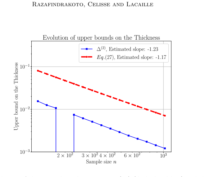
- [Theorem 34, Eq. (27), Appendix D.4] The refined thickness bound is proved by invoking Lemma 61 with beta = kappa^2 beta_{ell;1}/(lambda(n+1)). Lemma 61 requires beta < 1 for the contraction argument in Lemma 60 to apply. The theorem's assumption lambda(n+1) > kappa^2 beta_{ell;1}/2 only implies beta < 2. In the range kappa^2 beta_{ell;1}/2 < lambda(n+1) <= kappa^2 beta_{ell;1}, the maps h_i^lo/h_i^up are not guaranteed to be bijections, and the interval argument yielding 12T/(1-beta) breaks down. This is a genuine gap in the proof of the stated theorem, not a mere presentation issue; Corollary 35 inherits the problem. The rate is likely salvageable by strengthening the condition to lambda(n+1) > kappa^2 beta_{ell;1} or by a separate argument for the intermediate regime, but as written Theorem 34 is not proved in the claimed region.
- [Propositions 28 and 29, Appendix D.3] The proof of Proposition 28 selects epsilon satisfying the SmallEps conditions (Lemmas 51-52) and applies Lemma 55, which requires the map v |-> f_hat_lambda(v; .) to be twice continuously differentiable on an open neighborhood of [u,w]. The theorem statements do not mention these epsilon-conditions. Since a suitable epsilon always exists for lambda>0 and finite n, this is not a mathematical obstruction, but the proof's dependence on these conditions should be stated explicitly in the propositions (or the implicit choice of epsilon should be explained once).
minor comments (6)
- [Definition 4, Eq. (9)] The two inequalities in Eq. (9) compare S_tilde_Dy on both sides. The intended statement is |S_Dy - S_tilde_Dy| <= tau_i(y). This typo sits in the central definition and should be corrected.
- [Lemma 5, Theorem 12] The manuscript repeatedly misspells 'Theorem' as 'Thereom' in cross-references to Theorem 2. Please correct throughout.
- [Appendix B.1, proof of Theorem 11] For i=n+1 the proof concludes with the bound without the gamma factor: sqrt(K_i,i) sqrt(K_n+1,n+1) rho/(lambda(n+1)), whereas the theorem claims gamma rho. Since the score is gamma-Lipschitz, the gamma factor should appear; the same argument as for i<=n gives the claimed bound.
- [Lemmas 22-23, Definition 24] The notation I_f is overloaded: it denotes both a function in the RKHS and a vector in R^{n+1}. The distinction is explained, but the double use is likely to confuse readers; a different symbol for the vector representation would help.
- [Appendix D.1, Definition 50] Omega_epsilon is defined as an epsilon-neighborhood but the norm on R^{n+2} is not specified. Please state explicitly that the Euclidean norm is used.
- [Figure 2 caption] The caption contains the typo 'thiskness' in 'upper bound on the thiskness'.
Circularity Check
No circularity: thickness/covariance bounds are derived from explicit score-error inequalities; the result is not an input.
full rationale
The claimed derivation is not circular. The full conformal region is used only as the target to be sandwiched; the approximating region is built from explicitly bounded score approximations (Definition 4, Eqs. 9–11), and Lemma 7 sandwiches the true region using those bounds, with no thickness or coverage quantity appearing as an input. The stability-based bound (Theorem 12, Eq. 15) follows from the uniform bound τ^(0) and Lemma 38; the local-stability bound (Corollary 18) follows from τ^(1) ≤ τ^(0); the influence-function bound (Theorem 34, Eq. 27) follows from Proposition 28/Theorem 29 and Lemma 61 by plugging in the derivative estimate of y ↦ f̃^IF. The constants ρ, γ, ξℓ, κ, βℓ;1, βℓ;2 are assumed upper bounds, not fitted parameters, and λ and the anchor z are set a priori; the empirical slopes in Figures 1–10 are presented as checks against the theory, not calibrations. The only self-citation (Arlot & Celisse 2010) is a background survey on cross-validation and is not load-bearing; no uniqueness theorem, ansatz, or prior result of the authors is invoked to force the main conclusion. Corollary 31 omits a proof but the omission is indeed a direct application of Lemma 5 and Theorem 2. The threshold concern about Theorem 34 — that Lemma 61 requires β = κ²βℓ;1/(λ(n+1)) < 1 while the theorem only assumes λ(n+1) > κ²βℓ;1/2 — is a possible correctness/proof-regime issue, not a circularity, since the derived bound does not coincide with any input by construction.
Assumptions & free parameters
free parameters (3)
- ridge regularization λ =
λ ∝ (n+1)^{-0.33} in experiments; fixed in theory
- anchor output z =
z = 0 in all experiments
- loss scale a (and quantile level t) =
a=1.0 (logcosh, pseudo-Huber); a=0.2, t=5 (smoothed pinball)
assumptions (9)
- domain assumption Convexity of the loss in its second argument (ConvL), Assumption 8
- domain assumption Loss ρ-Lipschitz (ρ-LipL) and score γ-Lipschitz (γ-LipS), Assumptions 9–10
- domain assumption Smoothness C2L, C3L, (βℓ;2-LipDL.2), (ξℓ-BdD3), Assumptions 15, 21, 26, 27
- domain assumption Kernel finiteness (FinK) and boundedness (κ-BdK), Assumptions 20, 32
- ad hoc to paper SmallEps conditions, Lemmas 51–52 and Definition 50
- domain assumption Exchangeability of (X_1,Y_1),...,(X_{n+1},Y_{n+1}) and permutation invariance of f̂ (Theorem 2 assumptions)
- domain assumption Bounded conditional density p(·|D, X_{n+1}) ≤ c, Corollaries 13 and 35
- standard math Existence/uniqueness of the RKHS minimizer and Representer theorem, Lemma 44
- standard math Mean-value theorem in Hilbert spaces and the implicit function theorem, Lemmas 46–59
invented entities (1)
-
Thickness THK_α(X_{n+1})
Cite this review
Pith. "Pith review of Approximate full conformal prediction in an RKHS." pith.science (2026). https://pith.science/paper/HLMGKQRQ
@misc{pith2026260113102,
  author       = {Pith},
  title        = {Pith review of: Approximate full conformal prediction in an RKHS},
  year         = {2026},
  howpublished = {\url{https://pith.science/paper/HLMGKQRQ}},
  note         = {Machine review of arXiv:2601.13102}
}
read the original abstract
Full conformal prediction is a framework that implicitly formulates distribution-free confidence prediction regions for a wide range of estimators. However, a classical limitation of the full conformal framework is the computation of the confidence prediction regions, which is usually impossible since it requires training infinitely many estimators (for real-valued prediction for instance). The main purpose of the present work is to describe a generic strategy for designing a tight approximation to the full conformal prediction region that can be efficiently computed. Along with this approximate confidence region, a theoretical quantification of the tightness of this approximation is developed, depending on the smoothness assumptions on the loss and score functions. The new notion of thickness is introduced for quantifying the discrepancy between the approximate confidence region and the full conformal one.
Figures


Figures from the paper (7 more)




Reference graph
Works this paper leans on
-
[4]
Statistical properties of the log-cosh loss function used in machine learning
Resve A Saleh and AK Saleh. Statistical properties of the log-cosh loss function used in machine learning. arXiv preprint arXiv:2208.04564 ,
-
[2009]
Sublinear time low-rank approximation of positive semidefinite matrices
Cameron Musco and David P Woodruff. Sublinear time low-rank approximation of positive semidefinite matrices. In 2017 IEEE 58th Annual Symposium on Foundations of Computer Science (FOCS), pages 672–683. IEEE,
2017
-
[2015]
Conformalized kernel ridge regression
Evgeny Burnaev and Ivan Nazarov. Conformalized kernel ridge regression. In 2016 15th IEEE international conference on machine learning and applications (ICMLA) , pages 45–52. IEEE,
2016
-
[2016]
Valid selec- tion among conformal sets
Mahmoud Hegazy, Liviu Aolaritei, Michael I Jordan, and Aymeric Dieuleveut. Valid selec- tion among conformal sets. arXiv preprint arXiv:2506.20173 ,
-
[2022]
doi: https: //doi.org/10.10007/978-3-031-06649-8
ISBN 978-3-031-06648-1. doi: https: //doi.org/10.10007/978-3-031-06649-8. Shusen Wang, Alex Gittens, and Michael W Mahoney. Scalable kernel k-means cluster- ing with nystrom approximation: Relative-error bounds. Journal of Machine Learning Research, 20(12):1–49,
-
[2025]
Randomized algorithms for low-rank matrix approxi- mation: Design, analysis, and applications
Joel A Tropp and Robert J Webber. Randomized algorithms for low-rank matrix approxi- mation: Design, analysis, and applications. arXiv preprint arXiv:2306.12418 ,
Reviewed August 3, 2026 · model on record in the stance chip above.
Discussion (0). Sign in to comment.