REVIEW 4 major objections 6 minor 56 references
Diffusion-based annealed Boltzmann generators gain from second-order or deterministic transport-map corrections, but practical failures trace to learned log-density error, not score error.
Reviewed by Pith at T0; open to challenge. T0 means a machine referee read the full paper against a public rubric. the ladder, T0–T4 →
Even a perfect diffusion model yields poor annealed Boltzmann generators when coupled through first-order stochastic denoising kernels, while deterministic transport maps and second-order kernels improve; with learned densities, log-density error, not score error, is the bottleneck.
T0 review reviewed 2026-08-03 challenge →
load-bearing objection A useful idealized-regime decomposition and a promising deterministic transport variant, but the unbiased log-det claim is overstated and the 'systematic failure' headline runs ahead of the evidence. the 4 major comments →
Diffusion-based Annealed Boltzmann Generators : benefits, pitfalls and hopes
The pith
A machine-rendered reading of the paper's core claim, the machinery that carries it, and where it could break.
The reading
Core claim
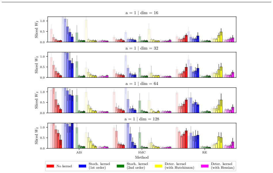
The systematic empirical study isolates inference effects from learning effects by comparing a perfectly learned diffusion model with one trained from data. With exact scores and log-densities, first-order stochastic denoising kernels—which only match the conditional mean—perform no better than a correlation-free baseline, whereas second-order Gaussian kernels that incorporate conditional covariance yield large gains. The paper then introduces deterministic transitions derived from the probability-flow ODE, built with an implicit midpoint integrator whose forward and backward maps are mutual inverses; estimating the Jacobian log-determinants via a power series and the Hutchinson trace trick
What carries the argument
The central object is the diffusion-induced density path together with the transition kernels/maps between adjacent noise levels: first-order stochastic denoising kernels (score-only), second-order stochastic kernels using Hessian-based covariance, and the newly proposed deterministic implicit-midpoint integrators of the probability-flow ODE, whose mutual invertibility and power-series Jacobian log-determinants (with Hutchinson trace estimation) make them usable inside AIS, SMC, and replica-exchange annealed samplers.
Load-bearing premise
The conclusion that log-density error, not score error, is the bottleneck assumes that the gap between the well-performing learned reverse dynamics and the failing annealed samplers is entirely due to log-density inaccuracy, and that the trained energy-based architectures and losses tested are representative of diffusion log-density estimation; if the hardcoded scores are imperfect at low temperature or the failures come from capacity or training instability rather than mode
What would settle it
Train a diffusion log-density model with an objective that provably recovers mode proportions (e.g., component-wise reweighting or a mode-aware regularizer) on the 16-mode Gaussian mixture, then rerun the AIS/SMC/RE comparisons; if performance jumps to idealized levels, the mode-blindness bottleneck is confirmed, and if not, it is falsified. For the idealized hierarchy, compute effective sample sizes for first-order versus second-order kernels on a two-mode Gaussian mixture with known exact conditional covariance; if first-order matches second-order, the claim that first-order kernels fail wou
If this is right
- Diffusion density paths should replace tempering paths in annealed samplers for multimodal targets, since they avoid abrupt mode switching and preserve relative mode weights.
- First-order stochastic denoising kernels are not worth the extra computation in diffusion-based annealed Boltzmann generators; second-order or deterministic transport-map corrections are required for meaningful gains.
- The deterministic transport-map framework provides a practical alternative to second-order methods, achieving comparable accuracy with only score information and a modest computational overhead.
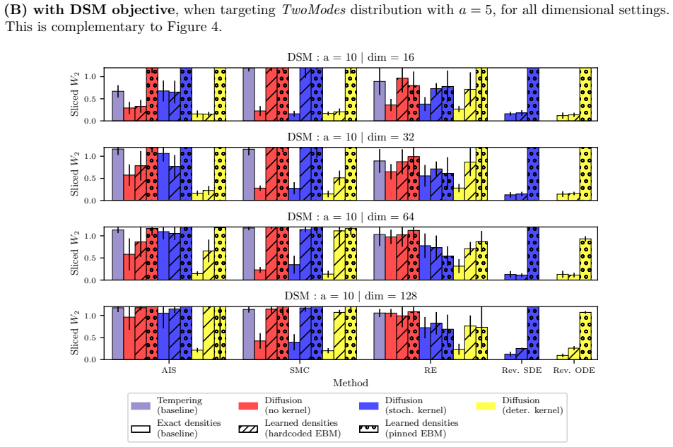
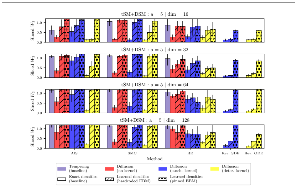
- In realistic settings, score accuracy is insufficient: annealed samplers fail because learned log-densities misrepresent mode proportions, even when the learned reverse dynamics are accurate.
- Training objectives that suffer from mode blindness will systematically disrupt SMC resampling and replica-exchange communication on multi-modal targets, dominating any benefit from improved transitions.
Where Pith is reading between the lines
- The Hutchinson-based log-determinant estimation could be adapted to other flow-based or transport-based samplers, offering an unbiased acceptance correction without explicit Hessians.
- The diagnosis points research toward log-density estimators that enforce correct mode weights; if such training schemes are developed, iterative diffusion-based annealed samplers could become viable.
- The mode-blindness mechanism likely affects any diffusion-based SMC or inference-time alignment algorithm that resamples using learned log-densities, even when the score is well learned.
Editorial analysis
A structured set of objections, weighed in public.
Referee Report
Summary. The paper studies diffusion-model-based annealed Monte Carlo Boltzmann Generators (DM-aMC-BGs) on controlled Gaussian-mixture targets, separating an idealized regime (exact scores and log-densities) from a realistic regime (learned energy-based parameterizations). It reports three main findings: (i) diffusion density paths generally outperform tempering paths in aMC; (ii) in the idealized regime, first-order stochastic denoising kernels give little or no improvement over a correlation-free baseline, while second-order stochastic kernels and a newly proposed deterministic transport-map integrator give substantial gains; and (iii) in the learned regime all DM-aMC-BG variants degrade, with the paper attributing the failure primarily to inaccurate, mode-blind DM log-density estimates rather than to learned scores. The paper includes a large appendix with proofs, additional experiments, and ablations, and the code is publicly available.
Significance. If its central claims hold, the paper makes a useful contribution: it provides a controlled benchmark that cleanly separates inference error from learning error, it identifies a concrete limitation of first-order stochastic denoising kernels inside aMC, it proposes a deterministic alternative that may be of independent interest, and it formulates a falsifiable hypothesis about mode blindness in DM log-density estimation. The strengths are the extensive idealized-regime experiments on Gaussian mixtures, the reproducible code release, and the unusually transparent discussion of limitations. However, the statistical-guarantee claim for the deterministic transport-map estimator is currently not correct as stated, and the empirical claims are stronger than the evidence presented in the figures. These issues bear directly on the headline conclusions and need to be addressed.
major comments (4)
- [§4.2, Prop. 3] The proposed Jacobian log-determinant estimator is not unbiased. The estimator truncates the power series at order I and replaces the implicit maps with finite-M fixed-point iterates. The Hutchinson estimator gives an unbiased estimate of each truncated trace term Tr([A^(M)]^i), not of log|det J|; no Russian-roulette debiasing is used. Therefore the log-det estimate has bias from truncation and from fixed-point error, and the importance weights in (21) and the acceptance probabilities in (22) are biased. The invocation of Andrieu & Roberts (2009) is not justified: pseudo-marginal MH requires an unbiased estimate of the weight/acceptance ratio, not of its logarithm. Since the central positive claim is that the deterministic transport map outperforms stochastic first-order variants, the reported advantage could be an artifact of this bias; the sensitivity to M and I shown in Figures 55-57
- [Fig. 3 / §3.3 / Abstract] The empirical support for the strong wording 'fail systematically' is insufficient. Figure 3 and the related figures show only averages over 8 runs with no error bars, standard deviations, or confidence intervals. The text in §3.3 is more cautious — 'do not yield noticeable improvements' — and the figure caption itself states that the first-order stochastic kernels 'does not always lead to better performance' than the baseline. Without uncertainty quantification, one cannot distinguish a systematic failure from statistical noise. Please report error bars or confidence intervals and align the abstract, §3.3, and the introduction with the actual strength of the empirical statement.
- [§6.2] The claim that the realistic-regime failure is 'not imputable to the quality of the learned scores, but rather to the learned log-densities' is a comparative inference, not a directly measured quantity. Figure 6 is a qualitative 1D visualization of learned density paths; no quantitative job-level error for learned log-densities versus learned scores is reported. Alternative explanations — for example network capacity, training instability (especially for the pinned architecture), or imperfect scores in low-temperature/tail regions — are not excluded. Since the 'bottleneck is inaccurate DM log-density estimation' message is one of the paper's main takeaways, please add quantitative diagnostics (e.g., mode-weight errors for the learned densities, score-error norms at intermediate levels), or perform ablations that hold one component fixed while varying the other, to isolate the claimed mec
- [§4.1-4.2] The finite fixed-point approximation also undermines the exactness of the deterministic aMC formulation itself. The derivation of the AIS weight (21) and the RE acceptance probability (22) relies on the mutual invertibility property (20). With M fixed-point iterations, the maps are not guaranteed to be mutual inverses, and the paper explicitly leaves the rejection-based safeguard to future work. Thus, even setting aside the log-det estimator bias, the implemented procedure is not the exact deterministic aMC described in §4.1. Please state this clearly and quantify the effect of M on the validity of the transport-map construction, or incorporate the rejection step so that the implemented algorithm matches the claimed statistical framework.
minor comments (6)
- [Abstract vs. §3.3] The abstract states that 'standard integrations using only first-order stochastic denoising kernels fail systematically,' while §3.3 says they 'do not yield noticeable improvements.' These are different claims; please use consistent wording.
- [Proof of Prop. 3, Eq. (34)] In the displayed equations, the second line writes log|det J_{T_{k+1|k}}(x_k)| where it should be log|det J_{T_{k|k+1}}(x_{k+1})|. Please correct the subscript.
- [§6.2] Typo: 'Harcoded' should be 'Hardcoded'.
- [Section C] The proof section says 'We leave the proof for the reader' for the EI-based VP/VE variants of the main propositions. These variants are used in the experiments, so either provide the proofs or state explicitly that they are direct substitutions and indicate where the required assumptions differ.
- [Abstract] The word 'meta-analysis' is unusual for a controlled empirical study with a new method. Consider replacing it with 'empirical study' or 'comparative analysis' to avoid implying a formal meta-analysis of the literature.
- [Figures 1 and 3] The figure captions note that darker bars correspond to larger K and that configurations do not share computational budget. This is important context but easy to miss; consider making it more prominent in the main-text discussion when claiming that diffusion paths 'outperform' tempering paths.
Circularity Check
No derivation in the paper reduces to its own inputs; the central findings are new controlled experiments. Minor self-citation to the authors' own benchmark targets is present but not load-bearing. A flagged correctness gap in Section 4.2 about the 'unbiased' Jacobian log-determinant estimator is a validity concern, not a circularity.
full rationale
Walking the derivation chain: in the idealized regime (Section 3 and 4), all intermediate log-densities, scores, and Hessians are computed exactly for Gaussian-mixture targets, so no fitted constant is reused as a prediction. The comparisons among first-order stochastic kernels, second-order stochastic kernels, and deterministic transports are empirical measurements on controlled benchmarks, not consequences of an equation that already contains the answer. The claimed advantage of deterministic transport is a new experimental finding, and its sensitivity to truncation/fixed-point hyperparameters is openly ablated (Figures 55–57). In the realistic regime (Section 6), the same network E_theta provides both the learned log-density and the learned score s_theta = -grad E_theta. The paper argues that since the learned reverse SDE/ODE (score-only) matches its ideal analog while the aMC variants (which additionally use E_theta values) fail, the bottleneck is inaccurate log-density estimation. This is a plausible statistical decomposition, but it is not a circular equivalence by construction: the score and the log-density are tied through one architecture, so a trajectory on which the score is accurate does not logically force the log-density level to be accurate elsewhere, and the conclusion depends on the representatives of the trained EBMs. This is a confounding/correctness risk, not a self-definitional reduction. The main self-referential elements are citations to the authors' own previous work for the benchmark targets (Grenioux et al. 2025; Noble et al. 2025) and for a Tweedie-style expansion (Grenioux et al. 2024). These are not used as uniqueness theorems or as smuggled ansatze; the target definitions are simply Gaussian-mixture densities, and the expansion is reproducible from the paper's own Lemmas 4–5 and Corollary 5. Thus the self-citations do not carry the derivational weight of the paper's claims. I flag one explicit validity gap, although it is not circularity: Section 4.2 calls the procedure an 'unbiased estimator, thereby preserving the statistical guarantees of aMC' and invokes Andrieu & Roberts (2009), but Proposition 3 is stated as an 'approximation' with a truncated power series (order I) and a finite fixed-point range (M). The Hutchinson estimator is unbiased for each truncated trace term, not for the untruncated log-determinant of the implicit-midpoint map; no Russian-roulette debiasing is used and the paper explicitly leaves it to future
Axiom & Free-Parameter Ledger
free parameters (3)
- K (number of annealing levels) =
optimized per method/target among {16, 32, 64, 128, 256}
- lambda_reg (regularization weight for LFPE/aLFPE/RNE) =
best of {1e-2, 1e-3, 1e-4} for LFPE/aLFPE and {10, 1, 0.1} for RNE
- M, I, NH (fixed-point iterations, truncation order, Hutchinson samples) =
M=4, I=3, NH=32
axioms (4)
- standard math Reverse-time SDE / PF-ODE formulation of diffusion models (Anderson 1982; Song et al. 2021) and Tweedie's formula for conditional denoising moments.
- ad hoc to paper Assumption 1/3: the score function is L_k-Lipschitz and the step size is small enough, δ_k = O(1/L_k), for the implicit midpoint fixed-point iteration to converge.
- domain assumption The controlled Gaussian mixture targets (TwoModes, ManyModes), standardized to zero mean and unit covariance, are adequate proxies for the multi-modal, high-barrier sampling problems encountered in molecular simulation.
- ad hoc to paper Mode blindness of score-based objectives (Wenliang & Kanagawa 2021) extends to TSM, tSM, LFPE, aLFPE, and RNE objectives and is the primary cause of the realistic-regime failure.
Cite this review
Pith. "Pith review of Diffusion-based Annealed Boltzmann Generators : benefits, pitfalls and hopes." pith.science (2026). https://pith.science/paper/YWZZUFRD
@misc{pith2026260121026,
  author       = {Pith},
  title        = {Pith review of: Diffusion-based Annealed Boltzmann Generators : benefits, pitfalls and hopes},
  year         = {2026},
  howpublished = {\url{https://pith.science/paper/YWZZUFRD}},
  note         = {Machine review of arXiv:2601.21026}
}
read the original abstract
Sampling configurations at thermodynamic equilibrium is a central challenge in statistical physics. Boltzmann Generators (BGs) tackle it by combining a generative model with a Monte Carlo (MC) correction step to obtain asymptotically unbiased samples from an unnormalized target. Most current BGs use classic MC mechanisms such as importance sampling, which both require tractable likelihoods from the backbone model and scale poorly in high-dimensional, multi-modal targets. We study BGs built on annealed Monte Carlo (aMC), which is designed to overcome these limitations by bridging a simple reference to the target through a sequence of intermediate densities. Diffusion models (DMs) are powerful generative models and have already been incorporated into aMC-based recalibration schemes via the diffusion-induced density path, making them appealing backbones for aMC-BGs. We provide an empirical meta-analysis of DM-based aMC-BGs on controlled multi-modal Gaussian mixtures (varying mode separation, number of modes, and dimension), explicitly disentangling inference effects from learning effects by comparing (i) a perfectly learned DM and (ii) a DM trained from data. Even with a perfect DM, standard integrations using only first-order stochastic denoising kernels fail systematically, whereas second-order denoising kernels can substantially improve performance when covariance information is available. We further propose a deterministic aMC integration based on first-order transport maps derived from DMs, which outperforms the stochastic first-order variant at higher computational cost. Finally, in the learned-DM setting, all DM-aMC variants struggle to produce accurate BGs; we trace the main bottleneck to inaccurate DM log-density estimation. Code available at https://github.com/h2o64/dabg.
Figures








Reference graph
Works this paper leans on
-
[1]
standardized
+ 1 3N(x;a1d,Σ 2), whereΣ 1, Σ2∈R d×d are diagonal covariance matrices. The diagonal entries ofΣ1 are given by(Σ1)i,i = i dσ2 max + d−i d σ2 min, and those ofΣ 2 are the reverse ofΣ 1:(Σ 2)i,i = (Σ 1)d−i,d−i, with σ2 max = 0.2and σ2 min = 0.01(hence, the conditioning number of each covariance matrix is20). We vary the separation parameter a∈{ 1.0, 2.5, 5....
2025
-
[2]
Proof.This is an immediate corollary from (Hall, 2000, Theorem 3.6)
For any matrixM∈R d×d satisfying∥M∥<min(1/|α|,1/|β|), the following identities hold log [ (Id−βM)−1(Id +αM) ] = ∞∑ i=1 βi−(−1)iαi i Mi,log [ (Id +βM)−1(Id−αM) ] = ∞∑ i=1 (−1)iβi−αi i Mi, wherelogdenotes the matrix logarithm. Proof.This is an immediate corollary from (Hall, 2000, Theorem 3.6). Corollary 5.Let( c1,c 2,c
2000
-
[3]
A.2 Discrete time setting for diffusion models Following Karras et al
Similar computations withM2 lead to the second result. A.2 Discrete time setting for diffusion models Following Karras et al. (2024); Grenioux et al. (2024), we define the time discretization{tk}K k=0⊂ [0,T ] accordingly to the growth (in log-scale) of the noise levelt↦→σ(t). 31 Given fixed boundary valuesσmin >0andσ max >0, we define for anyk∈{0,...,K}th...
2024
-
[6]
=dlog|c 1|+ log det ( (Id +c 2M)−1(Id−c 3M ) ) =dlog|c 1|+ Tr log ( (Id +c 2M)−1(Id−c 3M ) ).(Hall, 2000, Theorem 3.10) Hence, we obtain the first result of Corollary 5 by using the second statement of Lemma 4 withβ =c2 and α=c
2000
-
[8]
Gabriel Cardoso, Yazid Janati el idrissi, Sylvain Le Corff, and Eric Moulines
URL https://proceedings.neurips.cc/paper_files/paper/2024/file/ bcd11db0b26d8fc2266b91d3ff982ed1-Paper-Conference.pdf. Gabriel Cardoso, Yazid Janati el idrissi, Sylvain Le Corff, and Eric Moulines. Monte carlo guided denoising diffusion models for bayesian linear inverse problems. InThe Twelfth International Conference on Learning Representations,
2024
-
[9]
Ricky TQ Chen, Yulia Rubanova, Jesse Bettencourt, and David K Duvenaud
URL https://proceedings.neurips.cc/paper/2019/file/ 5d0d5594d24f0f955548f0fc0ff83d10-Paper.pdf. Ricky TQ Chen, Yulia Rubanova, Jesse Bettencourt, and David K Duvenaud. Neural ordinary differential equations.Advances in neural information processing systems,
2019
-
[13]
URLhttps://www.pnas.org/doi/abs/10.1073/pnas.2109420119
doi: 10.1073/pnas.2109420119. URLhttps://www.pnas.org/doi/abs/10.1073/pnas.2109420119. Ruiqi Gao, Yang Song, Ben Poole, Ying Nian Wu, and Diederik P Kingma. Learning energy-based models by diffusion recovery likelihood. InInternational Conference on Learning Representations,
-
[14]
Florentin Guth, Zahra Kadkhodaie, and Eero P Simoncelli
URL https: //openreview.net/forum?id=d91E9RhVFU. Florentin Guth, Zahra Kadkhodaie, and Eero P Simoncelli. Learning normalized image densities via dual score matching. InThe Thirty-ninth Annual Conference on Neural Information Processing Systems, 2025a. URLhttps://openreview.net/forum?id=wtYcS4kxpF. Florentin Guth, Zahra Kadkhodaie, and Eero P Simoncelli. ...
-
[16]
Jonathan Ho, Ajay Jain, and Pieter Abbeel
URLhttps://arxiv.org/abs/2506.05668. Jonathan Ho, Ajay Jain, and Pieter Abbeel. Denoising diffusion probabilistic models.Advances in neural information processing systems, 33:6840–6851,
-
[17]
Koji Hukushima and Koji Nemoto
URLhttps://arxiv.org/abs/2210.02303. Koji Hukushima and Koji Nemoto. Exchange monte carlo method and application to spin glass simulations. Journal of the Physical Society of Japan, 65(6):1604–1608,
-
[19]
D Experimental details D.1 Target details Definition of theTwoModestarget distribution.For our target π, we first consider the Gaussian mixture introduced in Grenioux et al
Similarly, one could use the coefficients from Proposition 25 for the VE noising scheme combined with exponential integration. D Experimental details D.1 Target details Definition of theTwoModestarget distribution.For our target π, we first consider the Gaussian mixture introduced in Grenioux et al. (2025), whose density is defined overRd as γ(x) = 2 3N(x;−a1d,Σ
2025
-
[20]
URLhttps://doi.org/10.1021/acs.jpclett.2c03327
doi: 10.1021/acs.jpclett.2c03327. URLhttps://doi.org/10.1021/acs.jpclett.2c03327. Yazid Janati, Badr Moufad, Alain Durmus, Eric Moulines, and Jimmy Olsson. Divide-and-conquer posterior sampling for denoising diffusion priors. In A. Globerson, L. Mackey, D. Belgrave, A. Fan, U. Paquet, J. Tomczak, and C. Zhang (eds.),Advances in Neural Information Processi...
-
[21]
Yazid Janati, Eric Moulines, Jimmy Olsson, and Alain Oliviero-Durmus
URL https://proceedings.neurips.cc/paper_files/ paper/2024/file/b0ae046e198a5e43141519868a959c74-Paper-Conference.pdf. Yazid Janati, Eric Moulines, Jimmy Olsson, and Alain Oliviero-Durmus. Bridging diffusion posterior sampling and monte carlo methods: a survey.Philosophical Transactions of the Royal Society A: Mathematical, Physical and Engineering Scienc...
2024
-
[22]
URLhttps: //royalsocietypublishing.org/doi/abs/10.1098/rsta.2024.0331
doi: 10.1098/rsta.2024.0331. URLhttps: //royalsocietypublishing.org/doi/abs/10.1098/rsta.2024.0331. Tero Karras, Miika Aittala, Timo Aila, and Samuli Laine. Elucidating the design space of diffusion-based generative models.Advances in Neural Information Processing Systems, 35:26565–26577,
arXiv 2024
-
[23]
Leon Klein, Andreas Krämer, and Frank Noé
URLhttps://proceedings.neurips.cc/ paper_files/paper/2024/file/5035a409f5798e188079e236f437e522-Paper-Conference.pdf. Leon Klein, Andreas Krämer, and Frank Noé. Equivariant flow matching.Neural Information Processing Systems (NeurIPS),
2024
-
[26]
ISSN 0730-0301, 1557-7368. doi: 10.1145/3341156. URLhttps://dl.acm.org/doi/10.1145/3341156. Radford M Neal. Annealed importance sampling.Statistics and computing, 11:125–139,
-
[28]
ISSN 0036-8075, 1095-9203. doi: 10.1126/science.aaw1147. URLhttps://www.science.org/doi/10.1126/science.aaw1147. Kaoru Ohno, Keivan Esfarjani, and Yoshiyuki Kawazoe.Computational Materials Science: From Ab Initio to Monte Carlo Methods. Springer,
-
[29]
doi: https://doi.org/10.1016/S0009-2614(01)00055-0
ISSN 0009-2614. doi: https://doi.org/10.1016/S0009-2614(01)00055-0. URL https://www.sciencedirect. com/science/article/pii/S0009261401000550. Bernt Øksendal. Stochastic differential equations. InStochastic differential equations: an introduction with applications, pp. 38–50. Springer,
-
[30]
URLhttp://www.jstor.org/ stable/3318418
ISSN 13507265. URLhttp://www.jstor.org/ stable/3318418. Tim Salimans and Jonathan Ho. Should EBMs model the energy or the score? InEnergy Based Models Workshop-ICLR 2021,
arXiv 2021
-
[31]
URL https: //arxiv.org/abs/2410.15336. Raghav Singhal, Zachary Horvitz, Ryan Teehan, Mengye Ren, Zhou Yu, Kathleen McKeown, and Rajesh Ranganath. A general framework for inference-time scaling and steering of diffusion models. InForty- second International Conference on Machine Learning,
-
[32]
Jeffrey Mark Siskind
URLhttps://openreview.net/forum?id= Jp988ELppQ. Jeffrey Mark Siskind. Automatic differentiation: Inverse accumulation mode. InProgram Transformations for ML Workshop at NeurIPS 2019,
2019
-
[33]
URLhttps://arxiv. org/abs/2101.03288. Yang Song, Jascha Sohl-Dickstein, Diederik P Kingma, Abhishek Kumar, Stefano Ermon, and Ben Poole. Score-based generative modeling through stochastic differential equations. InThe Ninth International Conference on Learning Representations,
-
[36]
URL https://rss.onlinelibrary.wiley.com/doi/abs/10.1111/rssb.12464
doi: https://doi.org/10.1111/rssb.12464. URL https://rss.onlinelibrary.wiley.com/doi/abs/10.1111/rssb.12464. Saifuddin Syed, Alexandre Bouchard-Côté, Kevin Chern, and Arnaud Doucet. Optimised annealed sequential monte carlo samplers,
-
[37]
James Thornton, Louis Béthune, Ruixiang ZHANG, Arwen Bradley, Preetum Nakkiran, and Shuangfei Zhai
URLhttps://arxiv.org/abs/2408.12057. James Thornton, Louis Béthune, Ruixiang ZHANG, Arwen Bradley, Preetum Nakkiran, and Shuangfei Zhai. Controlled generation with distilled diffusion energy models and sequential monte carlo. InThe 28th International Conference on Artificial Intelligence and Statistics,
-
[38]
URLhttps://arxiv.org/ abs/2407.13734. Pascal Vincent. A connection between score matching and denoising autoencoders.Neural computation, 23 (7):1661–1674,
-
[39]
URLhttps://arxiv.org/abs/2008.10087. 29 Luhuan Wu, Brian L. Trippe, Christian A Naesseth, John Patrick Cunningham, and David Blei. Practical and asymptotically exact conditional sampling in diffusion models. InThirty-seventh Conference on Neural Information Processing Systems,
Pith/arXiv arXiv 2008
-
[40]
Fengzhe Zhang, Jiajun He, Laurence I Midgley, Javier Antorán, and José Miguel Hernández-Lobato
URL https://openreview.net/forum?id=Gn2izAiYzZ. Fengzhe Zhang, Jiajun He, Laurence I Midgley, Javier Antorán, and José Miguel Hernández-Lobato. Efficient and unbiased sampling of boltzmann distributions via consistency models.arXiv preprint arXiv:2409.07323,
-
[41]
Midgley, and José Miguel Hernández-Lobato
Fengzhe Zhang, Laurence I. Midgley, and José Miguel Hernández-Lobato. Efficient and unbiased sampling from boltzmann distributions via variance-tuned diffusion models, 2025a. URLhttps://arxiv.org/abs/ 2505.21005. Leo Zhang, Peter Potaptchik, Jiajun He, Yuanqi Du, Arnaud Doucet, Francisco Vargas, Hai-Dang Dau, and Saifuddin Syed. Accelerated parallel tempe...
arXiv 2022
-
[45]
Define the matrices M1 =c 1(Id +c 2M)−1(Id−c 3M),M 2 =c−1 1 (Id−c 3M)−1(Id +c 2M)
LetM ∈R d×d be a matrix satisfying ∥M∥< min(1/|c 2|,1/|c 3|). Define the matrices M1 =c 1(Id +c 2M)−1(Id−c 3M),M 2 =c−1 1 (Id−c 3M)−1(Id +c 2M). Then we have log|det M 1|=dlog|c 1|+ ∞∑ i=1 (−1)ici 2−ci 3 i Tr[Mi],log|det M 2|=−dlog|c 1|+ ∞∑ i=1 ci 3−(−1)ici 2 i Tr[Mi]. Proof. Consider such(c1,c 2,c 3)and such matrixM. Note that the assumption onc2 and c3 ...
2019
-
[48]
DSM objective
Then, for any pair of time-steps(s,t )such thatT≥t>s≥0, the ODE solutionY t givenY s =y s∈R d is defined by Yt = exp (∫t s f(u)du ) ys + ( exp (∫t s f(u)du ) −1 ) b. Proof.Let0≤s<t≤T, setZ t = exp(−F(t))Yt, whereF(t) = ∫t 0f(u)du, then dZt =f(t) exp(−F(t))bdt, which implies that Zt =Z+ (exp(−F(s))−exp(−F(t)))b, which gives the result. 32 A.4 Review of sco...
2021
-
[49]
TSM objective
2 2 ] , withX t =S(t)X 0 +r(t)Z , X− t =S(t)X 0−r(t)Z. In our experiments, the “TSM objective” will systematically refer to the training loss function˜Lanti TSM. As originally proposed by Bortoli et al. (2024), this loss can also be combined with preconditioning schemes to reduce its variance in practice; however, since those are not compatible with the...
2024
-
[50]
Lemma 8(Exact noising SDE integration - General case).The conditional distribution of Xt given Xs =x s∈R d is defined by the Gaussian kernel qt|s(·|xs) = N ( {S(t)/S(s)}xs,S(t) 2{σ2(t)−σ 2(s)}Id ) , 9While He et al. (2025) propose to replaceqt|s, though tractable, by its Euler-Maruyama estimation, our implementation relies rather on its exact formulation ...
2025
-
[51]
Below, we present a rigorous expression of this upper bound onδ for the noising schemes considered in this paper, that is theVariance-Preservingapproach (see Section B.2) and theVariance-Explodingapproach (see Section B.3). B.2 Variance-Preserving diffusion Consider the noising SDE(2) where f(t) =−g2(t)/2and g being such that ∫T 0 g2(s)ds≫ 1, with arbitra...
2021
-
[52]
Then, SDE (2) simply writes as dXt =g(t)dW t, X0∼π .(31) This noising scheme is known as theVariance-Exploding(VE) scheme (Song et al., 2021). On the choice of theg-schedule.Following the guidelines from (Karras et al., 2022), we consider the geometric schedule g2(t) =σ 2 min (σ2 max σ2 min )t log (σ2 max σ2 min ) , whereσ min≈0andσ max≫1can be arbitraril...
2021
-
[55]
To evaluate how well mode weights are recovered, we compute the Total Variation (TV) distance between the true mode weight histogram and its Monte Carlo estimate
Moreover, we apply the same standardization procedure as for theTwoModestargets. To evaluate how well mode weights are recovered, we compute the Total Variation (TV) distance between the true mode weight histogram and its Monte Carlo estimate. D.2 Training and sampling parameters Diffusion model training details.As explained in Section 6.1, we consider tw...
2023
-
[56]
In particular, when training networks with TSM and RNE objectives, we initializeUθ based on the output of DSM training procedure
and set the default learning rate as10−4, multiplied by a factord−1 for score matching approaches (DSM, TSM, tSM) andd−2 for energy matching techniques (LFPE, aLFPE, RNE), following guidelines of related works. In particular, when training networks with TSM and RNE objectives, we initializeUθ based on the output of DSM training procedure. In the case of t...
2025
-
[1953]
ISSN 0021-9606. doi: 10.1063/1.1699114. URLhttps://doi.org/10.1063/1.1699114. L. I. Midgley, V. Stimper, G. N. C. Simm, and J. M. Hernández-Lobato. Bootstrap your flow. In1st ELLIS Machine Learning for Molecule Discovery Workshop, December
-
[1982]
doi: https://doi.org/10.1016/0304-4149(82)90051-5
ISSN 0304-4149. doi: https://doi.org/10.1016/0304-4149(82)90051-5. URLhttps: //www.sciencedirect.com/science/article/pii/0304414982900515. Christophe Andrieu and Gareth O. Roberts. The pseudo-marginal approach for efficient Monte Carlo computations.The Annals of Statistics, 37(2):697 – 725,
-
[1986]
URLhttps://link.aps.org/ doi/10.1103/PhysRevLett.57.2607
doi: 10.1103/PhysRevLett.57.2607. URLhttps://link.aps.org/ doi/10.1103/PhysRevLett.57.2607. Publisher: American Physical Society. Saifuddin Syed, Vittorio Romaniello, Trevor Campbell, and Alexandre Bouchard-Cote. Parallel tempering on optimized paths. In Marina Meila and Tong Zhang (eds.),Proceedings of the 38th International Conference on Machine Learnin...
-
[1987]
doi: https://doi.org/10.1016/0370-2693(87)91197-X
ISSN 0370-2693. doi: https://doi.org/10.1016/0370-2693(87)91197-X. URL https://www.sciencedirect.com/science/article/pii/037026938791197X. Daan Frenkel and Berend Smit.Understanding Molecular Simulation: from Algorithms to Applications. Elsevier,
-
[1989]
URLhttps://doi.org/10.1080/03610918908812806
doi: 10.1080/ 03610918908812806. URLhttps://doi.org/10.1080/03610918908812806. Aapo Hyvärinen. Estimation of non-normalized statistical models by score matching.Journal of Machine Learning Research, 6(24):695–709,
-
[1996]
URL https://doi.org/10.1143/JPSJ.65.1604
doi: 10.1143/JPSJ.65.1604. URL https://doi.org/10.1143/JPSJ.65.1604. M.F. Hutchinson. A stochastic estimator of the trace of the influence matrix for laplacian smoothing splines.Communications in Statistics - Simulation and Computation, 18(3):1059–1076,
-
[2000]
Jiajun He, José Miguel Hernández-Lobato, Yuanqi Du, and Francisco Vargas
URLhttps://arxiv.org/ abs/math-ph/0005032. Jiajun He, José Miguel Hernández-Lobato, Yuanqi Du, and Francisco Vargas. Rne: plug-and-play diffusion inference-time control and energy-based training,
-
[2001]
MCMC using hamiltonian dynamics.arXiv preprint arXiv:1206.1901,
Radford M Neal. MCMC using hamiltonian dynamics.arXiv preprint arXiv:1206.1901,
Pith/arXiv arXiv 1901
-
[2009]
URLhttps: //doi.org/10.1214/07-AOS574
doi: 10.1214/07-AOS574. URLhttps: //doi.org/10.1214/07-AOS574. Michael Arbel, Alex Matthews, and Arnaud Doucet. Annealed flow transport monte carlo. InInternational Conference on Machine Learning, pp. 318–330. PMLR,
-
[2010]
Jingtong Sun, Julius Berner, Lorenz Richter, Marius Zeinhofer, Johannes Müller, Kamyar Azizzadenesheli, and Anima Anandkumar. Dynamical measure transport and neural pde solvers for sampling.arXiv preprint arXiv:2407.07873, 2024a. Jingtong Sun, Julius Berner, Lorenz Richter, Marius Zeinhofer, Johannes Müller, Kamyar Azizzadenesheli, and Anima Anandkumar. D...
-
[2011]
ISSN 0004-5411. doi: 10.1145/1944345.1944349. URLhttps://doi.org/10.1145/1944345.1944349. Fan Bao, Chongxuan Li, Jiacheng Sun, Jun Zhu, and Bo Zhang. Estimating the optimal covariance with imperfect mean in diffusion probabilistic models. In Kamalika Chaudhuri, Stefanie Jegelka, Le Song, Csaba Szepesvari, Gang Niu, and Sivan Sabato (eds.),Proceedings of t...
-
[2016]
URLhttps://doi.org/10.1080/10618600.2015.1060885
doi: 10.1080/10618600.2015.1060885. URLhttps://doi.org/10.1080/10618600.2015.1060885. Yaxuan Zhu, Jianwen Xie, Ying Nian Wu, and Ruiqi Gao. Learning energy-based models by cooperative diffusion recovery likelihood. InThe Twelfth International Conference on Learning Representations,
arXiv 2015
-
[2017]
URLhttp://www.jstor.org/stable/26408299
ISSN 08834237, 21688745. URLhttp://www.jstor.org/stable/26408299. Tara Akhound-Sadegh, Jarrid Rector-Brooks, Joey Bose, Sarthak Mittal, Pablo Lemos, Cheng-Hao Liu, Marcin Sendera, Siamak Ravanbakhsh, Gauthier Gidel, Yoshua Bengio, Nikolay Malkin, and Alexander Tong. Iterated denoising energy matching for sampling from boltzmann densities. InProceedings of...
-
[2019]
doi: 10.1103/PhysRevD.100.034515
ISSN 2470-0010, 2470-0029. doi: 10.1103/PhysRevD.100.034515. URLhttps://link.aps.org/doi/10.1103/PhysRevD.100.034515. Brian D.O. Anderson. Reverse-time diffusion equation models.Stochastic Processes and their Applications, 12(3):313–326,
-
[2020]
doi: 10.1007/978-3-030-47845-2_8
ISBN 978-3-030-47845-2. doi: 10.1007/978-3-030-47845-2_8. URL https://doi.org/10.1007/978-3-030-47845-2_8. Luigi Del Debbio, Joe Marsh Rossney, and Michael Wilson. Machine Learning Trivializing Maps: A First Step Towards Understanding How Flow-Based Samplers Scale Up.PoS, LATTICE2021:059,
-
[2021]
URLhttps://arxiv.org/abs/2111. 11510. Laurence Midgley, Vincent Stimper, Javier Antorán, Emile Mathieu, Bernhard Schölkopf, and José Miguel Hernández-Lobato. Se(3) equivariant augmented coupling flows. In A. Oh, T. Naumann, A. Globerson, K. Saenko, M. Hardt, and S. Levine (eds.),Advances in Neural Information Processing Systems, volume 36, pp. 79200–79225...
2023
-
[2022]
Pierre Del Moral, Arnaud Doucet, and Ajay Jasra
doi: 10.22323/1.396.0059. Pierre Del Moral, Arnaud Doucet, and Ajay Jasra. Sequential monte carlo samplers.Journal of the Royal Statistical Society Series B: Statistical Methodology, 68(3):411–436,
-
[2023]
URLhttps://onlinelibrary.wiley.com/ doi/abs/10.1002/sta4.625
doi: https://doi.org/10.1002/sta4.625. URLhttps://onlinelibrary.wiley.com/ doi/abs/10.1002/sta4.625. Yan Zhou, Adam M. Johansen, and John A.D. Aston. Toward automatic model comparison: An adaptive sequential monte carlo approach.Journal of Computational and Graphical Statistics, 25(3):701–726,
-
[2024]
doi: 10.1038/s41586-024-07487-w
ISSN 1476-4687. doi: 10.1038/s41586-024-07487-w. URLhttps: //doi.org/10.1038/s41586-024-07487-w. S. Agapiou, O. Papaspiliopoulos, D. Sanz-Alonso, and A. M. Stuart. Importance sampling: Intrinsic dimension and computational cost.Statistical Science, 32(3):405–431,
-
[2025]
URLhttps: //arxiv.org/abs/2506.16471. M. S. Albergo, G. Kanwar, and P. E. Shanahan. Flow-based generative models for markov chain monte carlo in lattice field theory.Physical Review D, 100(3):034515, 8
This paper was first reviewed by deepseek-v4-flash on August 3, 2026.
discussion (0)
Sign in with ORCID, Apple, or X to comment. Anyone can read and Pith papers without signing in.