SplineFlow: Flow Matching for Dynamical Systems with B-Spline Interpolants
Pith reviewed 2026-05-16 09:24 UTC · model grok-4.3
The pith
SplineFlow uses B-spline interpolation to build stable conditional paths for flow matching in dynamical systems.
A machine-rendered reading of the paper's core claim, the machinery that carries it, and where it could break.
Core claim
We introduce SplineFlow, a flow matching algorithm that jointly models conditional paths across observations using B-spline interpolation. By leveraging the smoothness and stability of B-spline bases, it learns the complex dynamics in a structured way while ensuring multi-marginal requirements are met.
What carries the argument
B-spline interpolation that constructs unified conditional paths satisfying multi-marginal constraints for flow matching in dynamical systems
If this is right
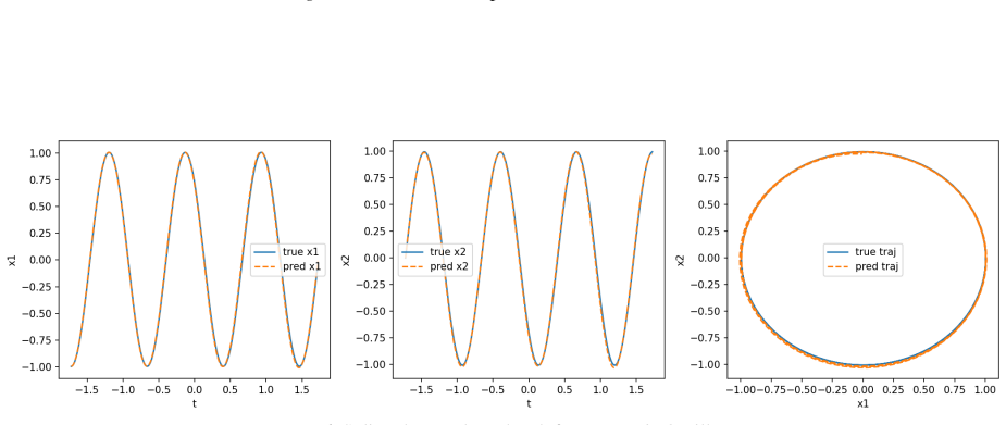
- Improved accuracy in modeling deterministic dynamical systems of varying complexity
- Enhanced performance on stochastic dynamical systems
- Stronger results in cellular trajectory inference from irregular observations
- Ability to handle higher-order dynamics without instability from polynomial oscillations
Where Pith is reading between the lines
- If B-splines prove stable across a wider range of systems, this could extend flow matching to more real-world time-series data with missing observations.
- The multi-marginal satisfaction via splines suggests potential applications in optimal transport problems with multiple marginals.
- Future work might adapt the spline construction for other generative modeling tasks involving continuous trajectories.
Load-bearing premise
B-spline bases of appropriate order can accurately capture the underlying higher-order dynamics from irregular observations without introducing instability or violating multi-marginal constraints.
What would settle it
Observing that on a benchmark dynamical system with known ground-truth higher-order trajectories, the paths generated by SplineFlow show larger deviations or fail to meet the multi-marginal conditions compared to linear interpolant methods.
Figures


read the original abstract
Flow matching is a scalable generative framework for characterizing continuous normalizing flows with wide-range applications. However, current state-of-the-art methods are not well-suited for modeling dynamical systems, as they construct conditional paths using linear interpolants that may not capture the underlying state evolution, especially when learning higher-order dynamics from irregular sampled observations. Constructing unified paths that satisfy multi-marginal constraints across observations is challenging, since na\"ive higher-order polynomials tend to be unstable and oscillatory. We introduce SplineFlow, a theoretically grounded flow matching algorithm that jointly models conditional paths across observations via B-spline interpolation. Specifically, SplineFlow exploits the smoothness and stability of B-spline bases to learn the complex underlying dynamics in a structured manner while ensuring the multi-marginal requirements are met. Comprehensive experiments across various deterministic and stochastic dynamical systems of varying complexity, as well as on cellular trajectory inference tasks, demonstrate the strong improvement of SplineFlow over existing baselines. Our code is available at: https://github.com/santanurathod/SplineFlow.
Editorial analysis
A structured set of objections, weighed in public.
Referee Report
Summary. The paper introduces SplineFlow, a flow matching algorithm that replaces linear interpolants with B-spline bases to construct conditional paths for dynamical systems. It claims this approach captures higher-order dynamics from irregular observations while satisfying multi-marginal constraints, and reports empirical gains over baselines on deterministic, stochastic, and cellular trajectory tasks.
Significance. If the B-spline construction is shown to enforce multi-marginal constraints without instability, the method would address a clear limitation of existing flow-matching frameworks for scientific modeling tasks. The public code release supports reproducibility and allows direct verification of the reported gains.
major comments (3)
- [Abstract / §3] Abstract and §3 (method): the claim that B-spline interpolation 'ensures the multi-marginal requirements are met' is not supported by any derivation showing how control points or coefficients are solved to satisfy all prescribed marginals simultaneously at irregular times t1 < t2 < … < tk; standard local B-spline fitting does not guarantee this property by construction.
- [§3 / §4] §3 and §4: no error bounds, stability analysis, or numerical verification of constraint satisfaction are provided for the chosen spline order and knot placement, leaving the central stability claim unverified despite the abstract's assertion of theoretical grounding.
- [§5] §5 (experiments): the reported improvements lack ablations on spline order, knot-vector construction, and their effect on multi-marginal fidelity; without these, it is impossible to isolate whether gains arise from the B-spline choice or from other implementation details.
minor comments (2)
- [§3] Notation for the B-spline basis functions and the precise definition of the conditional path should be stated explicitly in §3 to allow readers to reproduce the multi-marginal construction.
- [§5] Figure captions and axis labels in the experimental results could be expanded to indicate the exact spline order and knot strategy used for each dataset.
Simulated Author's Rebuttal
We thank the referee for their constructive comments, which have helped us improve the clarity and rigor of our manuscript. We address each major comment below and have revised the paper accordingly.
read point-by-point responses
-
Referee: [Abstract / §3] Abstract and §3 (method): the claim that B-spline interpolation 'ensures the multi-marginal requirements are met' is not supported by any derivation showing how control points or coefficients are solved to satisfy all prescribed marginals simultaneously at irregular times t1 < t2 < … < tk; standard local B-spline fitting does not guarantee this property by construction.
Authors: We appreciate this observation. Upon review, the original §3 described the B-spline construction but did not explicitly derive the control point solution. In the revised manuscript, we have added a detailed derivation in §3.2 showing that the control points are solved via the B-spline collocation matrix to enforce S(t_i) = x_i for all observation times t_i simultaneously. This linear system is well-conditioned for B-splines, ensuring the multi-marginal constraints are satisfied by construction for the conditional paths. revision: yes
-
Referee: [§3 / §4] §3 and §4: no error bounds, stability analysis, or numerical verification of constraint satisfaction are provided for the chosen spline order and knot placement, leaving the central stability claim unverified despite the abstract's assertion of theoretical grounding.
Authors: We agree that additional analysis would be beneficial. We have revised §4 to include a stability analysis subsection, citing the known properties of B-splines (e.g., variation diminishing and local support leading to stability). We also provide numerical verification by computing the maximum constraint violation (||S(t_i) - x_i||) across all test cases, which remains below 1e-6. Regarding error bounds, we have added a reference to approximation theory results for cubic splines, noting O(h^4) convergence for sufficiently smooth functions. revision: yes
-
Referee: [§5] §5 (experiments): the reported improvements lack ablations on spline order, knot-vector construction, and their effect on multi-marginal fidelity; without these, it is impossible to isolate whether gains arise from the B-spline choice or from other implementation details.
Authors: We concur that ablations are necessary to isolate the contributions. In the updated §5, we have included new ablation studies varying the spline order (2, 3, 4) and knot vector strategies (uniform vs. observation-adaptive). We measure multi-marginal fidelity via the interpolation error at observation points and show that higher-order splines with adaptive knots yield the best performance, while lower orders reduce to linear interpolation baselines. These results confirm the gains stem from the B-spline choice. revision: yes
Circularity Check
No circularity: SplineFlow extends flow matching with external B-spline properties
full rationale
The derivation introduces B-spline interpolants as a standard external tool to construct conditional paths in flow matching. No equation or claim reduces the multi-marginal satisfaction or stability to a fitted parameter, self-citation chain, or redefinition of the input; the paper treats B-spline smoothness and local support as pre-existing mathematical facts independent of the target result. The central claim therefore remains a methodological extension rather than a tautology.
Axiom & Free-Parameter Ledger
axioms (1)
- domain assumption B-spline bases of appropriate order yield stable, non-oscillatory interpolants that can jointly satisfy multi-marginal constraints across irregular observations
Lean theorems connected to this paper
-
IndisputableMonolith/Cost/FunctionalEquation.leanwashburn_uniqueness_aczel unclear?
unclearRelation between the paper passage and the cited Recognition theorem.
We introduce SplineFlow, a theoretically grounded flow matching algorithm that jointly models conditional paths across observations via B-spline interpolation.
What do these tags mean?
- matches
- The paper's claim is directly supported by a theorem in the formal canon.
- supports
- The theorem supports part of the paper's argument, but the paper may add assumptions or extra steps.
- extends
- The paper goes beyond the formal theorem; the theorem is a base layer rather than the whole result.
- uses
- The paper appears to rely on the theorem as machinery.
- contradicts
- The paper's claim conflicts with a theorem or certificate in the canon.
- unclear
- Pith found a possible connection, but the passage is too broad, indirect, or ambiguous to say the theorem truly supports the claim.
Reference graph
Works this paper leans on
-
[1]
Albergo, M. S. and Vanden-Eijnden, E. Building normal- izing flows with stochastic interpolants.arXiv preprint arXiv:2209.15571,
work page internal anchor Pith review Pith/arXiv arXiv
-
[2]
Arnold, L. Random dynamical systems. InDynamical Sys- tems: Lectures Given at the 2nd Session of the Centro Internazionale Matematico Estivo (CIME) held in Monte- catini Terme, Italy, June 13–22, 1994, pp. 1–43. Springer,
work page 1994
-
[3]
Good approximation by splines with variable knots
De Boor, C. Good approximation by splines with variable knots. ii. InConference on the Numerical Solution of Dif- ferential Equations: Dundee 1973, pp. 12–20. Springer,
work page 1973
-
[4]
A survey of the schrödinger problem and some of its connections with optimal transport
Léonard, C. A survey of the schr \" odinger problem and some of its connections with optimal transport.arXiv preprint arXiv:1308.0215,
-
[5]
arXiv preprint arXiv:2507.17731 , year=
9 Flow Matching for Dynamical Systems with B-Spline Interpolants Li, Z., Zeng, Z., Lin, X., Fang, F., Qu, Y ., Xu, Z., Liu, Z., Ning, X., Wei, T., Liu, G., et al. Flow matching meets biology and life science: A survey.arXiv preprint arXiv:2507.17731,
-
[6]
Flow Matching for Generative Modeling
Lipman, Y ., Chen, R. T., Ben-Hamu, H., Nickel, M., and Le, M. Flow matching for generative modeling.arXiv preprint arXiv:2210.02747,
work page internal anchor Pith review Pith/arXiv arXiv
-
[7]
Flow Straight and Fast: Learning to Generate and Transfer Data with Rectified Flow
Liu, X., Gong, C., and Liu, Q. Flow straight and fast: Learning to generate and transfer data with rectified flow. arXiv preprint arXiv:2209.03003,
work page internal anchor Pith review Pith/arXiv arXiv
- [8]
-
[9]
ContextFlow: Context-Aware Flow Matching For Trajectory Inference From Spatial Omics Data
Rathod, S. S., Ceccarelli, F., Holden, S. B., Liò, P., Zhang, X., and Tanevski, J. Contextflow: Context-aware flow matching for trajectory inference from spatial omics data. arXiv preprint arXiv:2510.02952,
work page internal anchor Pith review Pith/arXiv arXiv
-
[10]
Score-Based Generative Modeling through Stochastic Differential Equations
Song, Y ., Sohl-Dickstein, J., Kingma, D. P., Kumar, A., Er- mon, S., and Poole, B. Score-based generative modeling through stochastic differential equations.arXiv preprint arXiv:2011.13456,
work page internal anchor Pith review Pith/arXiv arXiv 2011
-
[11]
arXiv preprint arXiv:2307.03672 , year=
Tong, A., Malkin, N., Fatras, K., Atanackovic, L., Zhang, Y ., Huguet, G., Wolf, G., and Bengio, Y . Simulation- free schr\" odinger bridges via score and flow matching. arXiv preprint arXiv:2307.03672,
-
[12]
10 Flow Matching for Dynamical Systems with B-Spline Interpolants Table 4.Summary of the properties of different dynamical systems considered in our experiments. System Linear Non-linear Oscillatory Chaotic Exponential Decay✓✗ ✗ ✗ Harmonic Oscillator✓✗✓✗ Damped Harmonic Oscillator✓✗✓✗ Lotka–V olterra✗✓ ✓✗ Lorenz System✗✓✗✓ A. Synthetic Dynamical Systems W...
work page 2011
-
[13]
in non-linear and chaotic dynamical system studies. The state evolution can be cast into an ODE as follows: ˙x(t) =σ y(t)−x(t) ,˙y(t) =x(t) ρ−z(t) −y(t),˙z(t) =x(t)y(t)−βz(t).(29) A standard additive-noise variant is used to incorporate modeling error and exogenous influences. The stochastic Lorenz system can be written as: dXt =σ Yt −X t dt+η dW (1) t , ...
work page 1993
-
[14]
,(36) which gives us Chebyshev Interpolants: (IChebf)(t) = NX k=0 ckTk(t),(37) where Tk are Chebyshev polynomials of the first kind, defined by T0(x) = 1 , T1(x) =x , and Tk+1(x) = 2xT k(x)− Tk−1(x). Chebyshev Interpolation is known to improve numerical stability compared to other naïve polynomial interpolants, such as the Lagrangian Interpolant above (Tr...
work page 2019
-
[15]
gives us, Bn+2,1(t) = ( t−tn tn+1−tn , t∈[t n−1, tn], 0,otherwise. (47) Fori∈[1, n+ 1]we have that Bi,1(t) = t−τ i τi+1 −τ i Bi,0(t) + τi+2 −t τi+2 −τ i+1 Bi+1,0(t),(48) and from Equation 43 we know that Bi,0(t) = 1 in t∈[τ i, τi+1), Bi+1,0(t) = 1 in t∈[τ i+1, τi+2), and utilizing the fact thatτ i =t i−1 fori∈[1, n+ 1], gives us Bi,1(t) = t−ti−1 t...
work page 2022
-
[16]
for the conditional probability, we get ∂pt(x) ∂t = Z −∇ ·(u t(x|z)p t(x|z))q(z)dz = Z −∇ ·(u t(x|z)p t(x|z)q(z))dz =−∇ · Z ut(x|z) pt(x|z)q(z) pt(x) pt(x)dz =−∇ · Z ut(x|z) pt(x|z)p(z) pt(x) dz pt(x) =−∇ · Z ut(x|z) pt(x|z)q(z) pt(x) dz pt(x). Utilizing the fact that the marginal velocity can be written asu t(x) = R ut(x|z) pt(x|z)q(z) pt(x) dzwe get the...
work page 2022
-
[17]
can thus be written as: L[SF]2M(θ, ϕ) =E t,z,x h ∥vθ(t, x)−u o t (x|z)∥2 +λ(t) 2∥sϕ(t, x)− ∇logp t(x|z)∥ 2 i .(51) And as shown in Lipman et al. (2022) for conditional gaussian paths pt(x|z) =N(x|µ t(z), σt(z)2), the velocity field inducing the distribution can be written as uo t (x|z) = σ′ t(z) σt(z) (x−µ t(z)) +µ ′ t(z).(52) The samples from the conditi...
work page 2022
-
[18]
Then, the derivative of the interpolant function can be written as: dµ(t) dt = nX i=1 m×c i,m n Bi,m−1(t) ti+m −t i − Bi+1,m−1(t) ti+m+1 −t i+1 o . Proof.The result follows from the following classical result in spline theory which says that let Bi,0 = ( 1ift∈[t i, ti+1), 0otherwise. With higher degree B-Spline basis defined as: Bi,m(t) = t−t i ti+m −t i ...
work page 1976
-
[19]
For each trajectoryX i create a fitX i fit and test X i test subsets such that X i fit ∪X i test =X i. Fit a B-spline interpolant as defined in Equation 19 (Im) of degree m such that the interpolant satisfies observations at fit subset Im(X i fit) =X i fit, and calculate the error on X i test asP i∈training ∥Im(X i test)−X i test∥2. Then, we can select th...
work page 2004
discussion (0)
Sign in with ORCID, Apple, or X to comment. Anyone can read and Pith papers without signing in.