REVIEW 4 major objections 4 minor 37 references
This paper claims that 22 years of GRAPES-3 muon data separate the atmospheric-temperature and interplanetary-magnetic-field effects on muon flux, making the detector a dual monitor accurate to 10% and 6%.
Reviewed by Pith at T0; open to challenge. T0 means a machine referee read the full paper against a public rubric. the ladder, T0–T4 →
T0 review · deepseek-v4-flash
2026-08-02 23:56 UTC pith:VGAHUQEO
load-bearing objection Solid incremental measurement with an over-sold monitoring claim; deserves review but needs out-of-sample validation. the 4 major comments →
Monitoring the upper atmospheric temperature and interplanetary magnetic field with the GRAPES-3 muon telescope
The pith
A machine-rendered reading of the paper's core claim, the machinery that carries it, and where it could break.
Core claim
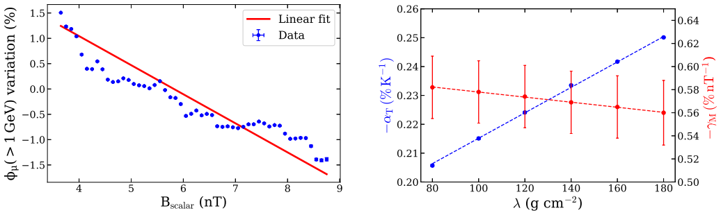
After correcting for atmospheric pressure and applying a 60-day running average, the authors isolate the annual component in both muon flux and effective temperature using a narrow band-pass filter centered on one cycle per year. They then iterate: correct the muon rate for the magnetic-field influence and refit the temperature coefficient, then correct for temperature and refit the magnetic-field coefficient. After three iterations the coefficients stabilize at αT = −0.2241 ± 0.0003 (stat.) ± 0.0220 (syst.) %/K and γM = −0.574 ± 0.027 (stat.) ± 0.011 (syst.) %/nT, for λ = 120 g/cm2. The paper states that the iteration removes the solar-cycle IMF modulation that otherwise leaks into the annu
What carries the argument
The key object is the effective temperature Teff: a weighted mean of the atmospheric temperature profile, with weights set by the hadronic attenuation length λ, which describes where cosmic-ray mesons interact and decay. The argument rides on an iterative frequency-domain fitting loop: a Fast Fourier Transform and a narrow band-pass filter isolate the one-year seasonal signal in the muon rate and in Teff; a linear fit gives the temperature coefficient; the muon rate is corrected by that coefficient; the residual is regressed against the scalar interplanetary magnetic-field magnitude measured at the L1 point; and the loop repeats until both coefficients converge. This machinery is what disent
Load-bearing premise
The load-bearing premise is that, after correcting for temperature, the remaining muon variation is a linear function of the scalar interplanetary magnetic-field magnitude measured at L1—and only that quantity—so the fitted γM would generalize outside the calibration period.
What would settle it
Hold out the most recent four years of the 22-year record, fit αT and γM on the earlier years, then use the muon rate to predict temperature and magnetic field in the held-out years; if the predictions do not match the reanalysis temperature and L1 magnetometer data within the claimed 10% and 6%, the monitor claim fails.
If this is right
- The telescope can serve as a long-term, ground-based check on upper-atmospheric temperature and L1 magnetic-field measurements, with stated accuracies of 10% and 6%.
- The final αT is about 23% larger in magnitude than the value obtained without the IMF iteration, so earlier estimates that omitted solar-cycle magnetic modulation are systematically low.
- The systematic uncertainty in both coefficients is dominated by the assumed hadronic attenuation length λ, quantified as ±0.022 %/K and ±0.011 %/nT for a 50 g/cm2 uncertainty in λ.
- If the coefficients are stable, the method can be extended to the telescope's directional bins and to future years, potentially giving a spatial picture of upper-atmosphere temperature changes.
- A validated γM would provide a ground-based monitor of interplanetary conditions that can fill gaps in spacecraft data at L1.
Where Pith is reading between the lines
- If the scalar-B linear model is incomplete, the fitted γM will partly absorb correlated solar-wind effects; a natural test is to fit with additional covariates such as solar-wind speed or field polarity and see whether γM shifts.
- The claimed 10% and 6% monitoring accuracies are in-sample; an out-of-sample test on data after 2022 would be the real bar for that statement.
- Applying the same iterative decomposition to muon telescopes at different latitudes could separate the common heliospheric signal from local atmospheric temperature, because the two components should scale differently between sites.
- With an independent IMF record, the method could be inverted to constrain the effective hadronic attenuation length of the atmosphere, since Teff weights depend on λ.
Editorial analysis
A structured set of objections, weighed in public.
Referee Report
Summary. The paper analyzes 22 years (2001–2022) of GRAPES-3 muon-telescope data, together with MERRA-2 effective atmospheric temperatures and L1 IMF magnitude from ACE/WIND, to derive linear response coefficients for upper-atmospheric temperature (α_T) and interplanetary magnetic field (γ_M). The analysis applies a 60-day running average, isolates the annual component with an FFT band-pass filter, and iteratively alternates between temperature and IMF corrections to converge on α_T = −0.2241 ± 0.0003 (stat.) ± 0.0220 (syst.) % K⁻¹ and γ_M = −0.574 ± 0.027 (stat.) ± 0.011 (syst.) % nT⁻¹ for λ = 120 g cm⁻². The paper then claims that GRAPES-3 can monitor upper-atmospheric temperature and the IMF to within 10% and 6%, respectively.
Significance. If the monitoring claim is substantiated, the result would be valuable: the 22-year high-statistics record, the automated detector-stability correction, and the iterative FFT-based decomposition are genuine strengths, and the final α_T is consistent with earlier GRAPES-3 results and theoretical expectations. The method is clearly described and the dataset is unique. However, the central claim of a long-term monitor is currently an extrapolation from in-sample fits; the paper does not provide an out-of-sample validation or an end-to-end inversion test. The reported statistical uncertainties also appear to ignore the strong serial correlation introduced by the running average and narrow band-pass filter.
major comments (4)
- [§4.1–4.3, Eqs. (3), (6), Figs. 8, 17, 18] The statistical uncertainties (e.g., α_T = −0.2241 ± 0.0003 % K⁻¹, γ_M = −0.574 ± 0.027 % nT⁻¹) are derived from fits to a large number of 3-hour points after a 60-day running average and a narrow band-pass filter with Δf = 1/T. The effective independent information is only about 22 annual cycles, so the raw point count drastically understates the uncertainty. Please compute errors using the effective number of independent samples (e.g., from the autocorrelation function or by bootstrapping yearly segments) and report the result; this is essential before the claimed precision can be accepted.
- [§5, opening sentence and abstract] The statement that GRAPES-3 'can serve as a long term monitor of both the upper atmospheric temperature and the interplanetary magnetic field to within 10% and 6%' is not demonstrated. The coefficients and the means used in Eqs. (3) and (6) are estimated from the full 2001–2022 record; no holdout validation or real-time inversion test is shown. A real-time monitor would require a stable baseline and must predict unseen periods. I recommend a concrete end-to-end test: fit on one part of the data (e.g., 2001–2011) and predict the muon-rate residuals for the remaining decade, reporting the RMS of inferred versus measured T_eff and B_scalar.
- [§4.2, Eq. (6)] The IMF monitor is built on a single-driver linear model where the temperature-corrected muon residual is a function only of B_scalar. Solar-cycle modulation of GCRs is known to depend on other correlated heliospheric quantities (solar-wind speed, magnetic polarity/tilt, rigidity-dependent diffusion). The fitted γ_M may therefore absorb these drivers and may not transfer outside the calibration period. To support the physical interpretation and the monitoring claim, add residual checks against V_sw and polarity, or a multivariate regression; alternatively, state explicitly that γ_M is a purely empirical calibration coefficient valid only for interpolation within the fitted conditions.
- [§3, pressure correction] The pressure coefficient is fixed to β = −0.128 %/hPa from Ref. [24], but no uncertainty is quoted or propagated. Since pressure has a strong annual cycle at this site, an error in β directly mimics the annual temperature signal and can bias α_T, which is a central result. Please quote the uncertainty on β and propagate it into α_T and γ_M, or show that the results are insensitive to a plausible range of β.
minor comments (4)
- [Abstract vs. body] The abstract states α_T = −0.2241 ± 0.04 (stat.) % K⁻¹, while the body and tables report ±0.0003 (stat.). This discrepancy should be corrected.
- [§4.3 and Table 2] The text says α_T and γ_M 'converge for all values of λ', but Table 2 shows α_T varying by about 20% across λ = 80–180 g cm⁻². The intended meaning is that iteration to convergence is achieved for each λ; please rephrase to avoid implying λ-independence of α_T.
- [Figures] Several figure axis labels contain encoding artifacts such as 'ϕ/uni03BC' (e.g., Figs. 4, 5, 7, 8, 10, 11, 15–18). The figures should be recompiled with correct muon and ΔT_eff symbols.
- [§1 and §5] The introduction says the data span 'three solar cycles,' but §5 correctly says 'parts of three solar cycles.' Use consistent wording.
Circularity Check
Monitoring accuracy (10%/6%) is quoted from the in-sample fitted coefficients, not an out-of-sample validation; the core coefficient measurement itself is a legitimate empirical fit.
specific steps
-
fitted input called prediction
[Section 5 'Summary of results' (monitoring claim); Eqs. (3) and (6) in Sections 4.1/4.2]
"These results demonstrate the potential of the GRAPES-3 muon telescope to serve as a long term monitor of both the upper atmospheric temperature and the interplanetary magnetic field to within 10% and 6% respectively."
The claimed monitoring accuracy is not validated out-of-sample; it is simply the relative uncertainty of the same fitted coefficients. The quoted 10% matches the relative uncertainty of α_T (0.0220/0.2241 ≈ 9.8%) and the quoted 6% matches the combined relative uncertainty of γ_M (≈0.038/0.574 ≈ 6.6%). Equations (3) and (6) are inverted to infer T or B from the muon rate, so the monitor's stated accuracy is just the calibration's own parameter uncertainty. No holdout period, end-to-end inversion, or independent comparison is provided, making the monitoring capability an in-sample restatement of the fit rather than an independent prediction.
full rationale
The main coefficient measurements are not circular: α_T and γ_M are empirical fits of the GRAPES-3 muon rate against independent external data (MERRA-2 effective temperature and OMNI IMF magnitude), and the alternating iterative procedure is a standard backfitting/self-consistent estimation scheme rather than a definitional equivalence. The T_eff weighting follows standard effective-temperature formalism, and the pressure coefficient is taken from separate earlier work; the self-citation to the detector-efficiency correction algorithm [22] is a methodological dependence but is not used to define the target result. The genuine circular element is the monitoring claim: the demonstrated 'accuracy' reduces to the precision of the fitted calibration coefficients themselves, with no out-of-sample or end-to-end validation. This warrants a partial-circularity score of 6, while noting that the underlying coefficient determinations retain independent empirical content.
Axiom & Free-Parameter Ledger
free parameters (6)
- Temperature coefficient alpha_T =
-0.2241 %/K (lambda=120, iteration 3)
- IMF coefficient gamma_M =
-0.574 %/nT (lambda=120, iteration 3)
- Hadronic attenuation length lambda =
120 g/cm2 central; varied 80-180
- Pressure coefficient beta =
-0.128 %/hPa
- 60-day running-average window =
60 days
- Band-pass filter half-width Delta f =
0.000125 CPD (=1/T)
axioms (5)
- domain assumption Linear superposition: muon flux fractional variation = alpha_T * Delta_T_eff + gamma_M * Delta_B (Eqs. 3 and 6).
- ad hoc to paper The annual band-pass filtered muon signal is purely temperature-driven after IMF correction.
- domain assumption B_scalar at L1 is the single heliospheric driver of long-term cosmic-ray modulation relevant here.
- domain assumption Effective temperature with a single hadronic attenuation length lambda (Eq. 1) captures the atmospheric influence on muon flux.
- standard math FFT and band-pass filtering reconstruct the annual component without spectral leakage.
read the original abstract
We study the influence of variations in the upper atmospheric temperature and interplanetary magnetic field on the cosmic ray induced atmospheric muon flux measured by the GRAPES-3 experiment over 22 years (2001--2022) of data; spanning three solar cycles: the declining phase of Solar Cycle 23, the full Cycle 24, and the rising and maximum phases of Cycle 25. Located in Ooty- India, the GRAPES-3 large area (560\,$m^2$) muon telescope detects $\sim$4 billion muons daily above 1\,GeV, with an angular resolution of $\sim$4$^\circ$, enabling a statistical precision $<$0.01\% on the hourly muon rate. After accounting for the effect of atmospheric pressure variations, we compare this data with the upper atmospheric temperature inferred from NASA's MERRA-2 dataset as well as magnetic field data from the ACE and WIND spacecraft at Lagrange point L1. A simultaneous iterative fitting method employing Fast Fourier Transforms and a narrow band-pass filter reveals the temperature and magnetic field coefficients to be $\alpha_T=-\,0.2241\,\pm\,0.04\, (stat.)\,\pm\,0.0220\, (syst.)\,\%\,K^{-1}$ and $\gamma_{M}=-\,0.574\,\pm\,0.027\, (stat.)\,\pm\,0.011\, (syst.)\,\%\,\text{nT}^{-1}$, respectively, for an assumed hadronic attenuation length $\lambda$=120 g cm$^{-2}$, underscoring the potential of the GRAPES-3 muon telescope to serve as a real time monitor of the upper atmospheric temperature or interplanetary magnetic field.
Figures



Reference graph
Works this paper leans on
-
[1]
S. E. Forbush, World-Wide Cosmic-Ray V ariations, 1937- 1952, Journal of Geophysical Research 59 (4) (1954) 525–542. doi:10.1029/JZ059i004p00525
-
[2]
K. Badruddin, Anand, Study of the Forbush Decreases, Geomagnetic Storms, and Ground-Level Enhancements in Selected Intervals and Their Space Weather Implica- tions, Solar Physics 290 (4) (2015) 1271–1283. doi: 10.1007/s11207-015-0665-4
-
[3]
K. P . Arunbabu, H. M. Antia, S. R. Dugad, S. K. Gupta, Y . Hayashi, S. Kawakami, P . K. Mohanty, A. Oshima, P . Subramanian, How are Forbush decreases related to interplanetary magnetic field enhancements?, Astronomy and Astrophysics 580 (2015) A41. arXiv:1504.06473, doi:10.1051/0004-6361/201425115
Pith/arXiv arXiv 2015
-
[4]
P . K. Mohanty, D. Atri, S. R. Dugad, S. K. Gupta, B. Har- iharan, Y . Hayashi, A. Jain, S. Kawakami, S. D. Mor- ris, P . K. Nayak, A. Oshima, B. S. Rao, Solar diurnal anisotropy measured using muons in GRAPES-3 exper- iment in 2006, Pramana 81 (2) (2013) 343–357. doi: 10.1007/s12043-013-0561-0
-
[5]
V enkatesan, Badruddin, Cosmic-Ray Intensity V aria- tions in the 3-DIMENSIONAL Heliosphere, Space Sci- ence Reviews 52 (1-2) (1990) 121–194
D. V enkatesan, Badruddin, Cosmic-Ray Intensity V aria- tions in the 3-DIMENSIONAL Heliosphere, Space Sci- ence Reviews 52 (1-2) (1990) 121–194. doi:10.1007/ BF00704241
1990
-
[6]
M. S. Potgieter, Solar Modulation of Cosmic Rays, Living Reviews in Solar Physics 10 (1) (2013) 3. arXiv:1306. 4421, doi:10.12942/lrsp-2013-3
-
[7]
T. K. Gaisser, R. Engel, E. Resconi, Cosmic Rays and Particle Physics, 2016
2016
-
[8]
Greisen, Cosmic Ray Showers, Annual Review of Nuclear and Particle Science 10 (1960) 63–108
K. Greisen, Cosmic Ray Showers, Annual Review of Nuclear and Particle Science 10 (1960) 63–108. doi: 10.1146/annurev.ns.10.120160.000431
arXiv 1960
-
[9]
The L3 Collaboration, Measurement of the Atmospheric Muon Spectrum from 20 to 3000 GeV, arXiv e-prints (2004) hep–ex /0408114arXiv:hep-ex/0408114, doi: 10.48550/arXiv.hep-ex/0408114
-
[10]
R. L. Workman, V . D. Burkert, V . Crede, E. Klempt, U. Thoma, L. Tiator, K. Agashe, G. Aielli, B. C. Allanach, C. Amsler, M. Antonelli, E. C. Aschenauer, D. M. As- ner, H. Baer, S. Banerjee, R. M. Barnett, L. Baudis, C. W. Bauer, J. J. Beatty, V . I. Belousov, J. Beringer, A. Bet- tini, O. Biebel, K. M. Black, E. Blucher, R. Bonventre, V . V . Bryzgalov,...
2022
-
[11]
M. A. Shea, Book Review: Cosmic rays at Earth Re- searcher’s reference manual and data book. ISBN: 0-444- 59710-8; 1112 pages, hardbound; 190.59 Euro, 2001, Advances in Space Research 28 (12) (2001) 1773–1774. doi:10.1016/S0273-1177(01)00545-2
-
[12]
Hayashi, Y
Y . Hayashi, Y . Aikawa, N. V . Gopalakrishnan, S. K. Gupta, N. Ikeda, N. Ito, A. Jain, A. V . John, S. Karthikeyan, S. Kawakami, H. Kojima, T. Matsuyama, D. K. Mohanty, P . K. Mohanty, S. D. Morris, T. Non- aka, A. Oshima, B. S. Rao, K. C. Ravindran, M. Sasano, K. Sivaprasad, B. V . Sreekantan, H. Tanaka, S. C. Ton- war, K. Viswanathan, T. Y oshikoshi, A...
2005
-
[13]
P . H. Barrett, L. M. Bollinger, G. Cocconi, Y . Eisenberg, K. Greisen, Interpretation of Cosmic-Ray Measurements Far Underground, Reviews of Modern Physics 24 (3) (1952) 133–178. doi:10.1103/RevModPhys.24.133
-
[14]
Ambrosio, R
MACRO Collaboration, M. Ambrosio, R. Antolini, G. Auriemma, R. Baker, A. Baldini, G. C. Barbarino, B. C. Barish, G. Battistoni, R. Bellotti, C. Bemporad, P . Bernardini, H. Bilokon, V . Bisi, C. Bloise, T. Bosio, C. Bower, S. Bussino, F. Cafagna, M. Calicchio, D. Cam- pana, M. Carboni, M. Castellano, S. Cecchini, F. Cei, V . Chiarella, A. Corona, S. Coutu...
1997
-
[15]
E. W. Grashorn, Observation of Seasonal V ariations with the MINOS Far Detector, in: International Cosmic Ray Conference, V ol. 5 of International Cosmic Ray Confer- ence, 2008, pp. 1233–1236. arXiv:0710.1616, doi: 10.48550/arXiv.0710.1616
work page internal anchor Pith review Pith/arXiv arXiv doi:10.48550/arxiv.0710.1616 2008
-
[16]
P . Desiati, Seasonal V ariations of High Energy Cosmic Ray Muons Observed by the IceCube Observatory as a Probe of Kaon /Pion Ratio, in: International Cosmic Ray Conference, V ol. 1 of International Cosmic Ray Confer- ence, 2011, p. 78. doi:10.7529/ICRC2011/V01/0662
-
[17]
P . Adamson, I. Anghel, A. Aurisano, G. Barr, M. Bishai, A. Blake, G. J. Bock, D. Bogert, S. V . Cao, C. M. Castromonte, S. Childress, J. A. B. Coelho, L. Cor- win, D. Cronin-Hennessy, J. K. de Jong, A. V . De- van, N. E. Devenish, M. V . Diwan, C. O. Escobar, J. J. Evans, E. Falk, G. J. Feldman, T. H. Fields, M. V . Frohne, H. R. Gallagher, R. A. Gomes, ...
Pith/arXiv arXiv 2014
-
[18]
K. P . Arunbabu, S. Ahmad, A. Chandra, S. R. Dugad, S. K. Gupta, B. Hariharan, Y . Hayashi, P . Jagadeesan, A. Jain, V . B. Jhansi, S. Kawakami, H. Kojima, P . K. Mohanty, S. D. Morris, P . K. Nayak, A. Oshima, B. S. Rao, L. V . Reddy, S. Shibata, K. Tanaka, M. Zuberi, De- pendence of the muon intensity on the atmospheric tem- perature measured by the GRA...
doi:10.1016/j 2017
-
[19]
S. K. Gupta, Y . Aikawa, N. V . Gopalakrishnan, Y . Hayashi, N. Ikeda, N. Ito, A. Jain, A. V . John, S. Karthikeyan, S. Kawakami, T. Matsuyama, D. K. Mohanty, P . K. Mohanty, S. D. Morris, T. Nonaka, A. Oshima, B. S. Rao, K. C. Ravindran, M. Sasano, K. Sivaprasad, B. V . Sreekantan, H. Tanaka, S. C. Tonwar, K. Viswanathan, T. Y oshikoshi, GRAPES-3—A high-...
2005
-
[20]
P . K. Mohanty, K. P . Arunbabu, T. Aziz, S. R. Dugad, S. K. Gupta, B. Hariharan, P . Jagadeesan, A. Jain, S. D. Morris, B. S. Rao, Y . Hayashi, S. Kawakami, A. Oshima, S. Shibata, S. Raha, P . Subramanian, H. Kojima, Tran- sient weakening of earth’s magnetic shield probed by a cosmic ray burst , Phys. Rev. Lett. 117 (2016) 171101. doi:10.1103/PhysRevLett...
-
[21]
B. Hariharan, et al., Measurement of the Electrical Properties of a Thundercloud Through Muon Imaging by the GRAPES-3 Experiment, Phys. Rev. Lett. 122 (2019) 105101. arXiv:1903.09801, doi:10.1103/ PhysRevLett.122.105101
Pith/arXiv arXiv 2019
-
[22]
Paul, et al., An automated algorithmic method to mitigate long-term variations in the e fficiency of the GRAPES-3 muon telescope (5 2025)
S. Paul, et al., An automated algorithmic method to mitigate long-term variations in the e fficiency of the GRAPES-3 muon telescope (5 2025). arXiv:2505. 16440
2025
-
[23]
URL https://www.vaisala.com/en/measurement/ pressure
V alsala barometers. URL https://www.vaisala.com/en/measurement/ pressure
-
[24]
P . K. Mohanty, S. Ahmad, H. M. Antia, K. P . Arunbabu, A. Chandra, S. R. Dugad, S. K. Gupta, B. Hariharan, Y . Hayashi, P . Jagadeesan, A. Jain, S. Kawakami, H. Ko- jima, S. D. Morris, P . K. Nayak, A. Oshima, B. S. Rao, L. V . Reddy, S. Shibata, Fast Fourier transform to mea- sure pressure coe fficient of muons in the GRAPES-3 ex- periment, Astroparticle ...
-
[25]
I. G. Usoskin, G. A. Kovaltsov, I. A. Mironova, A. J. Tylka, W. F. Dietrich, Ionization e ffect of solar par- ticle GLE events in low and middle atmosphere, At- mospheric Chemistry & Physics 11 (5) (2011) 1979–
2011
-
[26]
Global Modeling and Assimilation O ffice (GMAO), inst3_3d_asm_np: Merra-2 3d, instantaneous, pressure-level, meteorology fields (3-hourly, 0.625ˇrx0.5ˇr, 72 levels), version 5.12.4 (2015). doi:10.5067/QBZ6MG944HW0. URL https://doi.org/10.5067/QBZ6MG944HW0
-
[27]
C. W. Smith, J. L’Heureux, N. F. Ness, M. H. Acuña, L. F. Burlaga, J. Scheifele, The ACE Magnetic Fields Experiment, Space Science Reviews 86 (1998) 613–632. doi:10.1023/A:1005092216668
-
[28]
R. P . Lepping, M. H. Ac ˜una, L. F. Burlaga, W. M. Far- rell, J. A. Slavin, K. H. Schatten, F. Mariani, N. F. Ness, F. M. Neubauer, Y . C. Whang, J. B. Byrnes, R. S. Kennon, P . V . Panetta, J. Scheifele, E. M. Worley, The Wind Mag- netic Field Investigation, Space Science Reviews 71 (1-4) (1995) 207–229. doi:10.1007/BF00751330
-
[29]
J. H. King, N. E. Papitashvili, Solar wind spatial scales in and comparisons of hourly Wind and ACE plasma and magnetic field data, Journal of Geophysical Research (Space Physics) 110 (A2) (2005) A02104. doi:10. 1029/2004JA010649
2005
-
[30]
A. N. Dmitrieva, R. P . Kokoulin, A. A. Petrukhin, D. A. Timashkov, Corrections for temperature effect for ground- based muon hodoscopes, Astroparticle Physics 34 (6) (2011) 401–411. doi:10.1016/j.astropartphys. 2010.10.013. 12
-
[31]
I. Riádigos, D. García-Castro, D. González-Díaz, V . Pérez-Muñuzuri, Atmospheric temperature ef- fect in secondary cosmic rays observed with a 2m2 ground-based trpc detector , Earth and Space Science 7 (9) (2020) e2020EA001131, e2020EA001131 10.1029 /2020EA001131. arXiv: https://agupubs.onlinelibrary.wiley.com/ doi/pdf/10.1029/2020EA001131, doi:https: //d...
-
[32]
A. H. Maghrabi, S. A. Alzahrani, A. S. Alruhaili, The Role of Atmospheric Pressure, Temperature, and Humid- ity on Cosmic Ray Muons at a Low Latitude Station, In- ternational Journal of Astronomy and Astrophysics 13 (3) (2023) 236–258. doi:10.4236/ijaa.2023.133014
arXiv 2023
-
[33]
M. Philippov, V . Makhmutov, G. Bazilevskaya, F. Zagu- mennov, V . Fomenko, Y . Stozhkov, A. Orlov,Accounting for meteorological e ffects in the detector of the charged component of cosmic rays, Geoscientific Instrumentation, Methods and Data Systems 10 (2) (2021) 219–226. doi:10.5194/gi-10-219-2021 . URL https://gi.copernicus.org/articles/10/ 219/2021/
-
[34]
M. Savic, A. Dragi, D. Maleti, N. V eselinovi, D. Jokovi, R. Banjanac, V . Udovii, D. Knezevi, New empirical meth- ods for correction of meteorological e ffects on cosmic ray muons, PoS ICRC2021 (2021) 1252. doi:10.22323/1. 395.1252
doi:10.22323/1 2021
-
[35]
S. Seetha, S. Megala, Aditya-L1 mission, Current Sci- ence 113 (4) (2017) 610. doi:10.18520/cs/v113/i04/ 610-612
-
[36]
T. Palmer, The ecmwf ensemble prediction system: Looking back (more than) 25years and projecting forward 25years , Quarterly Journal of the Royal Meteorological Society 145 (S1) (2019) 12–24. arXiv:https://rmets.onlinelibrary.wiley. com/doi/pdf/10.1002/qj.3383, doi:https: //doi.org/10.1002/qj.3383. URL https://rmets.onlinelibrary.wiley.com/ doi/abs/10.100...
doi:10.1002/qj.3383 2019
-
[1988]
doi:10.5194/acp-11-1979-201110.5194/ acpd-10-30381-2010
Pith/arXiv arXiv 1979
discussion (0)
Sign in with ORCID, Apple, or X to comment. Anyone can read and Pith papers without signing in.