REVIEW 1 major objections 6 minor 4 references
For linear shock-compression data, the paper shows that a standard non-informative prior makes the posterior of the Hugoniot parameters a bivariate t-distribution, so analysts can sample exact pressure–volume Hugoniot bands without MCMC.
Reviewed by Pith at T0; open to challenge. T0 means a machine referee read the full paper against a public rubric. the ladder, T0–T4 →
Bayesian linear regression yields an analytic t-distribution posterior for C0 and S, which can be sampled and pushed through Rankine-Hugoniot equations to obtain pressure-volume Hugoniot credible intervals.
T0 review reviewed 2026-08-02 challenge →
load-bearing objection A solid, honest tutorial that repackages textbook Bayesian linear regression into a practical recipe for sampling Hugoniot P-V curves, with real code and a transparent but not fully addressed particle-velocity error limitation. the 1 major comments →
A Tutorial on Bayesian Analysis of Linear Shock Compression Data
The pith
A machine-rendered reading of the paper's core claim, the machinery that carries it, and where it could break.
The reading
Core claim
The central claim is that under the likelihood Yi = C0 + S xi + εi with i.i.d. Gaussian errors and the improper prior p(β,σ²) ∝ 1/σ², the marginal posterior of β=(C0,S) is the bivariate t-distribution t2(βhat, Σ, n−2), where βhat is the least-squares estimate and Σ=s²(X'X)^{-1}. Thus all uncertainty about the Hugoniot parameters is captured by three known quantities: the least-squares center, the scale matrix, and the degrees of freedom. Samples are obtained exactly by drawing a standard normal vector and an independent chi-square variable and transforming; each sample is one linear Hugoniot, and propagation through the Rankine-Hugoniot conservation equations turns it into a P–V curve. The p
What carries the argument
The load-bearing object is the conjugate normal-inverse-gamma factorization of the joint posterior: β given σ² is normal with mean βhat and covariance σ²(X'X)^{-1}, while σ² marginally is inverse gamma. Integrating σ² out yields the bivariate t posterior for β, which is the exact distribution that carries all inference. Sampling uses β = L Z sqrt(ν/W) + βhat with Z a standard bivariate normal, W a chi-square with ν=n−2 degrees of freedom, and L a Cholesky factor of Σ. This identity is what makes the full pipeline—posterior, credible regions, predictive intervals, and P–V Hugoniot ensembles—available in closed form and computationally trivial.
Load-bearing premise
All measurement error is assumed to live in the shock velocity, with particle velocities known exactly; if particle velocities are themselves uncertain, the estimated slope is biased toward zero and the entire Hugoniot curve is displaced.
What would settle it
Generate synthetic datasets from a known linear Hugoniot with added noise on both Us and Up, then apply the paper's exact posterior. If the 95% credible band for the P–V curve excludes the generating curve well more than 5% of the time—because the slope is attenuated—the central assumption is refuted. A simpler single-case check: corrupt Up with noise in an existing dataset and watch whether the posterior slope moves below the value recovered when Up is treated as exact.
If this is right
- All posterior means and intervals reduce to the familiar least-squares numbers, so adopting the Bayesian approach does not cost the analyst the standard Hugoniot fit.
- Any number of Hugoniot curves in the pressure–volume plane can be drawn exactly and independently, making downstream equation-of-state fitting and hydrocode input straightforward.
- Credible intervals for interpolated shock velocity are widest far from the mean particle velocity and shrink with sample size, giving a rule of thumb for where experiments add information.
- Posterior predictive checks give a straightforward visual test of whether the Gaussian linear model matches the scatter in the observed shock data.
- The stability comparison with bootstrapping shows that variation in the bootstrap estimate of S for copper is driven partly by whether the extreme point is resampled, whereas the Bayesian posterior changes less when that point is removed.
Where Pith is reading between the lines
- If particle-velocity measurements carry realistic error, the posterior slope is attenuated toward zero and the whole P–V band shifts; the tutorial's closed-form bands are therefore best treated as conditional on exact-Up, not as a full error budget.
- The same conjugate argument applies to polynomial Hugoniots—quadratic or cubic models simply enlarge β and reduce degrees of freedom—so the tutorial effectively provides a free benchmark against which MCMC-based error models can be checked.
- Because the posterior is exact and the computation is trivial, the paper's recipe could be used as a default cross-check whenever a future analysis on the same datasets reports wider or narrower uncertainty from a more complex method.
Editorial analysis
A structured set of objections, weighed in public.
Referee Report
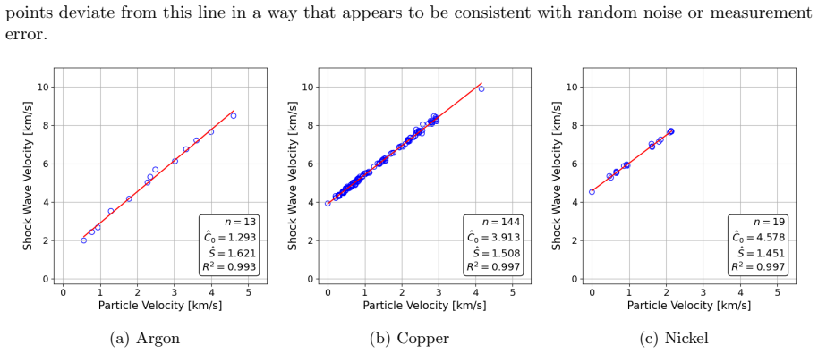
Summary. The paper is a tutorial on Bayesian uncertainty quantification for the empirical linear Hugoniot relation Us = C0 + S Up. It shows that, under a Gaussian likelihood with a non-informative prior on (beta, sigma^2), the marginal posterior of beta is a bivariate t-distribution centered at the OLS estimate (Sec. 3, Eq. 17). It then propagates samples of beta through the Rankine-Hugoniot equations to produce credible intervals for Hugoniot curves in the pressure-volume plane (Sec. 4), and also derives posterior predictive distributions for future shock-velocity measurements. The methodology is demonstrated on argon, copper, and nickel datasets from Marsh (1980), compared with nonparametric bootstrapping, and accompanied by publicly available reproducible code. The paper is explicitly pedagogical and does not claim new statistical methodology.
Significance. If taken with its stated modeling assumptions, the paper fills a useful pedagogical gap. The closed-form t posterior makes the tutorial self-contained and computationally inexpensive; the sampling procedure is exact; the code and data are public; and the posterior predictive checks are a sensible model-validation addition. The comparison with bootstrapping is instructive, and the authors are transparent that they are comparing different inferential objects. The central statistical derivation is standard and appears correct. The tutorial's main value is as an entry point and benchmark for more general UQ of Hugoniot data, and it is likely to be useful to practitioners new to Bayesian methods.
major comments (1)
- [Sec. 2, Eq. (2); Sec. 6, point 2; Eq. (17); Fig. 5] The load-bearing assumption that particle velocity Up is measured exactly is not a harmless simplification for the targeted experiments. Because the posterior in Eq. (17) is centered at the OLS estimate, any attenuation of the slope from x-error shifts the entire Hugoniot curve and the P-V credible bands in Fig. 5. The manuscript acknowledges the issue in Sec. 6, point 2, but does not quantify it, while the abstract and Sec. 2 (Eq. (2), 'effectively captures all sources of experimental uncertainty') frame the procedure as full measurement-uncertainty propagation. I ask for either (a) a sensitivity analysis in which plausible Up errors (e.g., 1-2% of Up) are added to the three datasets and the resulting changes in the posterior and P-V bands are reported, or (b) a consistent and prominent reframing of the tutorial, including the abstract, as conditional on Up being error-free. Without one
minor comments (6)
- [Sec. 2, text after Eq. (2)] The phrase 'effectively captures all sources of experimental uncertainty' is in tension with Sec. 6, point 2, which correctly notes that Up measurement error attenuates the regression slope. Please rephrase to avoid implying that the single Us error term absorbs Up error.
- [Appendix H, text after Eq. (H30)] The marginal posterior of beta is stated as a bivariate t-distribution 'with mean ~b'; the mean should be the vector beta-tilde, not the scale parameter b-tilde.
- [Appendix I, Fig. 14] The description says prediction intervals are obtained by adding normally distributed random variables 'with variances 2'. This appears to be a typo; it should be a clearly defined variance, presumably s^2 or a stated bootstrap residual variance.
- [Sec. 2, copper dataset description] The removal of one duplicate copper point is based on the authors' judgment and is disclosed, but the sensitivity of the reported summaries to this exclusion is not assessed. A one-sentence note or reference to a supplementary analysis would strengthen the reproducibility of the tutorial.
- [Sec. 5 and Conclusion] The claim that the Bayesian procedure is 'less sensitive' to the high-velocity copper point should be phrased carefully: the posterior distribution and the bootstrap sampling distribution answer different questions, and the difference in sensitivity is partly a consequence of that difference rather than a general methodological advantage. The current text is clear in Sec. 5, but the abstract and conclusion could overstate the point.
- [Sec. 4, Fig. 5] The shaded bands are described as '95% credible intervals for pressure as a function of volume.' It would be helpful to state explicitly that these are pointwise credible intervals rather than a joint credible band for the entire curve.
Circularity Check
No significant circularity: the tutorial derives a standard Bayesian linear-regression posterior and propagates it through the Rankine-Hugoniot equations without reducing its claims to fitted inputs or self-citations.
full rationale
The paper's central derivation (Sec. 3, Eqs. 6-17) is a self-contained application of standard Bayesian linear regression: a Gaussian likelihood (Eq. 8) combined with a non-informative prior (Eq. 9) yields a normal-inverse-gamma posterior, and integrating out the error variance gives the bivariate t-distribution of Eq. (17). The posterior mean equals the least-squares estimate (Eq. 18), a known identity that the paper explicitly acknowledges rather than presenting as an independent prediction. The downstream pressure-volume credible bands (Sec. 4, steps 1-3) are obtained by exact sampling from this posterior and propagating through the Rankine-Hugoniot conservation equations (Eqs. 23-24); this is uncertainty propagation, not a fitted input disguised as a prediction. The comparisons against ordinary linear regression and nonparametric bootstrapping are external benchmarks, and the bootstrap is shown to give broadly similar intervals, which supports rather than assumes the Bayesian result. Self-citations (Lindquist et al. 2023; Brown et al. 2023; Myint et al. 2023; Lindquist et al. 2024) appear only as contextual examples of MCMC-based EOS calibration and do not carry the derivation; the key statistical result is attributed to external statistics references (Gelman, Rencher-Schaalje, Banerjee). The paper also states in Sec. 2 and Sec. 6 that particle velocity is assumed known exactly and discusses attenuation bias from particle-velocity measurement error, so the main modeling limitation is disclosed rather than hidden. No load-bearing step reduces, by construction or self-citation, to its own inputs; the appropriate finding is no significant circularity.
Axiom & Free-Parameter Ledger
free parameters (2)
- Bootstrap prediction-interval noise variance =
2
- Copper duplicate-point removal =
removed
axioms (5)
- domain assumption Particle velocities Up are measured exactly; all measurement error enters Us as iid Gaussian noise.
- domain assumption The relationship Us = C0 + S Up is linear for the argon, copper, and nickel datasets.
- standard math The improper prior p(beta, sigma^2) ∝ 1/sigma^2 yields a proper posterior.
- domain assumption Rankine-Hugoniot conservation equations (mass and momentum) are valid for these materials.
- domain assumption The Marsh (1980) published datasets are accurate and internally consistent.
Cite this review
Pith. "Pith review of A Tutorial on Bayesian Analysis of Linear Shock Compression Data." pith.science (2026). https://pith.science/paper/S7C3VS6C
@misc{pith2026260305961,
  author       = {Pith},
  title        = {Pith review of: A Tutorial on Bayesian Analysis of Linear Shock Compression Data},
  year         = {2026},
  howpublished = {\url{https://pith.science/paper/S7C3VS6C}},
  note         = {Machine review of arXiv:2603.05961}
}
read the original abstract
Gas gun and other shock compression experiments often produce shock wave velocity measurements that are linearly associated with particle velocity. Traditionally, this empirical relationship is quantified with a single Hugoniot curve that is estimated using least squares regression. However, for downstream modeling and simulation tasks, it is often more useful to have multiple Hugoniot curves in the pressure-volume plane that are consistent with the data. We employ Bayesian uncertainty quantification methods as a framework for propagating measurement uncertainty through to model parameters and predictions. Specifically, this tutorial shows how to sample multiple Hugoniot curves in the pressure-volume plane that are consistent with the shock wave-particle velocity measurements in a two-step Bayesian approach. First, we obtain an analytical expression for the posterior distribution of the linear model parameters using Bayesian linear regression. Second, we propagate samples from the posterior distribution through the Rankine-Hugoniot equations to yield Hugoniot curves in the pressure-volume plane. The procedure is demonstrated with publicly available data on argon, copper, and nickel, and compared against bootstrapping and linear regression. The Bayesian procedure is shown to be interpretable, computationally inexpensive, and less sensitive than an alternative bootstrapping approach to the removal of the point in the copper dataset that has the largest particle velocity. As a tutorial on Bayesian methodology for the shock compression community, we provide several derivations and explanations that make this paper self-contained, and made all code and data available at https://github.com/llnl/BALSCD.
Figures



Reference graph
Works this paper leans on
-
[1]
and Stegun, I
Abramowitz, M. and Stegun, I. A. (1948).Handbook of mathematical functions with formulas, graphs, and mathematical tables, volume
1948
-
[5]
University of California Press. More, R. M., Warren, K. H., Young, D. A., and Zimmerman, G. B. (1988). A new quotidian equation of state (QEOS) for hot dense matter.Phys. Fluids, 31:3059–3078. Myint, P. C., Root, S., Wu, C. J., Clay, R. C., Lopez, A., Hanshaw, H. L., Lemke, R. W., Bliss, D. E., Hanson, D. L., Flicker, D. G., and Long, Z. C. (2023). Fluid-...
1988
-
[55]
US Government printing office. Ahrens, T. J. (1993). Equation of state. InHigh-Pressure Shock Compression of Solids, pages 75–113. Springer. Ali, S., Swift, D., Wu, C., and Kraus, R. (2020). Development of uncertainty-aware equation-of-state models: Application to copper.Journal of Applied Physics, 128(18). Banerjee, S. (2008). Bayesian linear model: Gory...
Pith/arXiv arXiv 1993
-
[526]
Hofert, M. (2013). On sampling from the multivariate t distribution.The R Journal, 5(2):129–136. Huijser, D., Goodman, J., and Brewer, B. J. (2022). Properties of the affine-invariant ensemble sampler’s ’stretch move’ in high dimensions.Australian & New Zealand Journal of Statistics, 64(1):1–26. Levashov, P. R., Khishchenko, K. V., Lomonosov, I. V., and F...
2013
This paper was first reviewed by deepseek-v4-flash on August 2, 2026.
discussion (0)
Sign in with ORCID, Apple, or X to comment. Anyone can read and Pith papers without signing in.