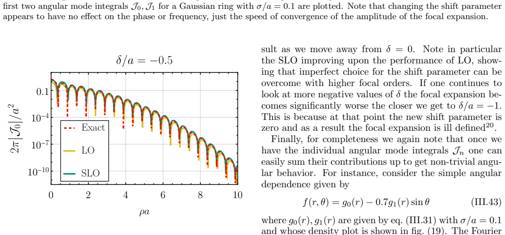
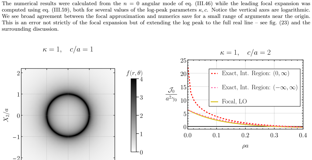
Approximating the Fourier Transform of Ring-Like Images: the Focal Expansion
Pith reviewed 2026-05-10 18:35 UTC · model grok-4.3
The pith
A single focal expansion term approximates the Fourier transforms of ring-like images accurately across small and large spatial frequencies.
A machine-rendered reading of the paper's core claim, the machinery that carries it, and where it could break.
Core claim
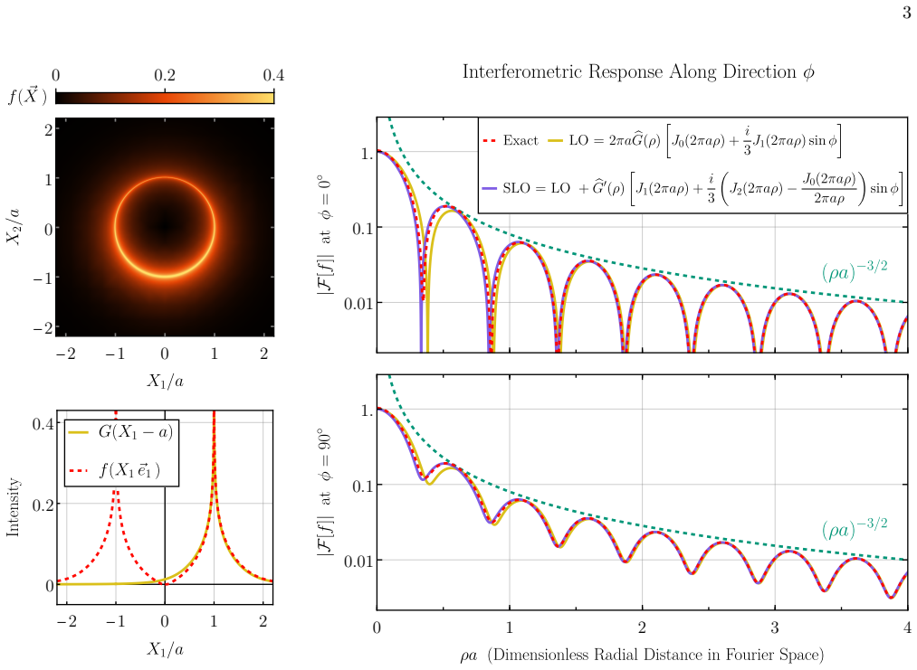
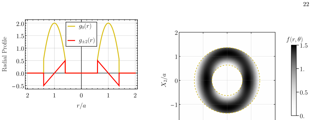
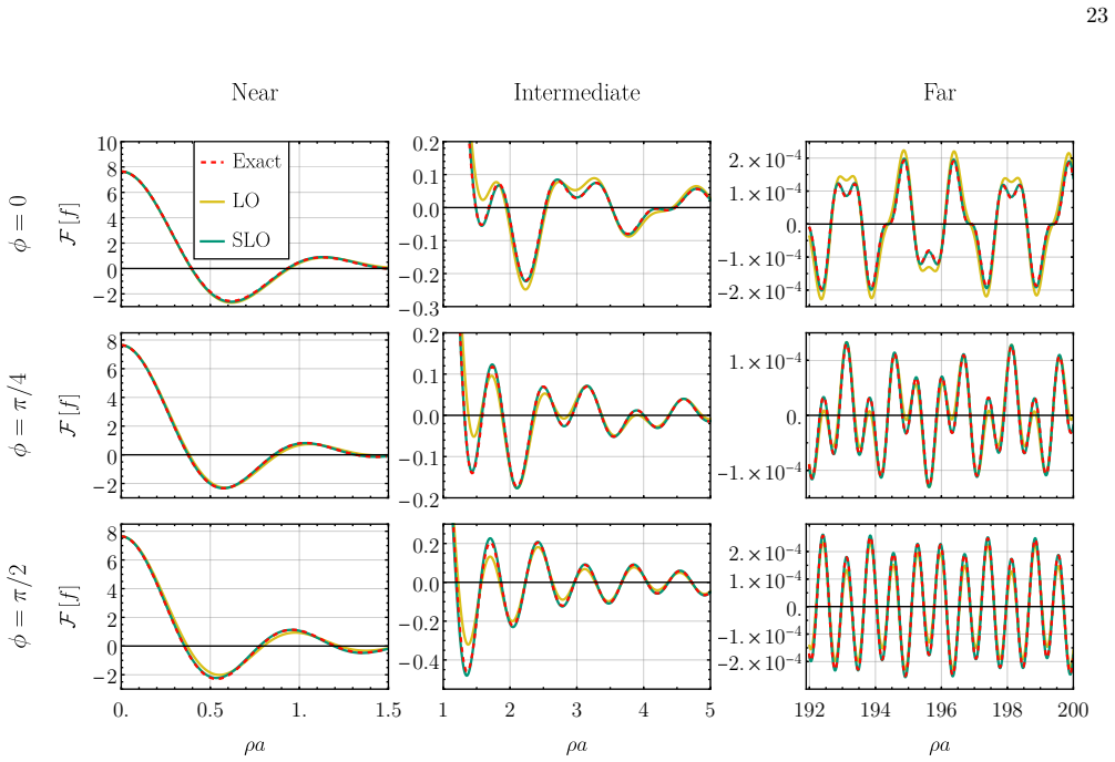
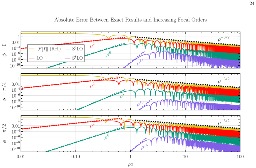
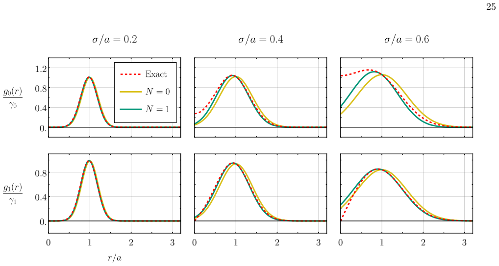
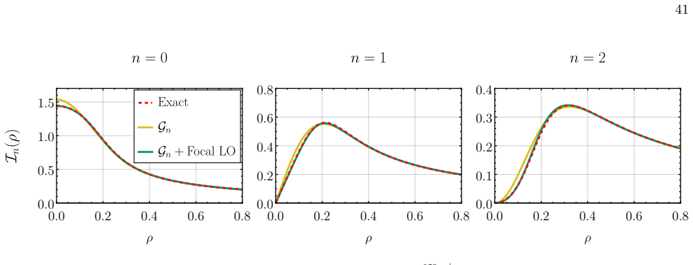
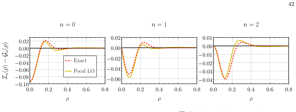
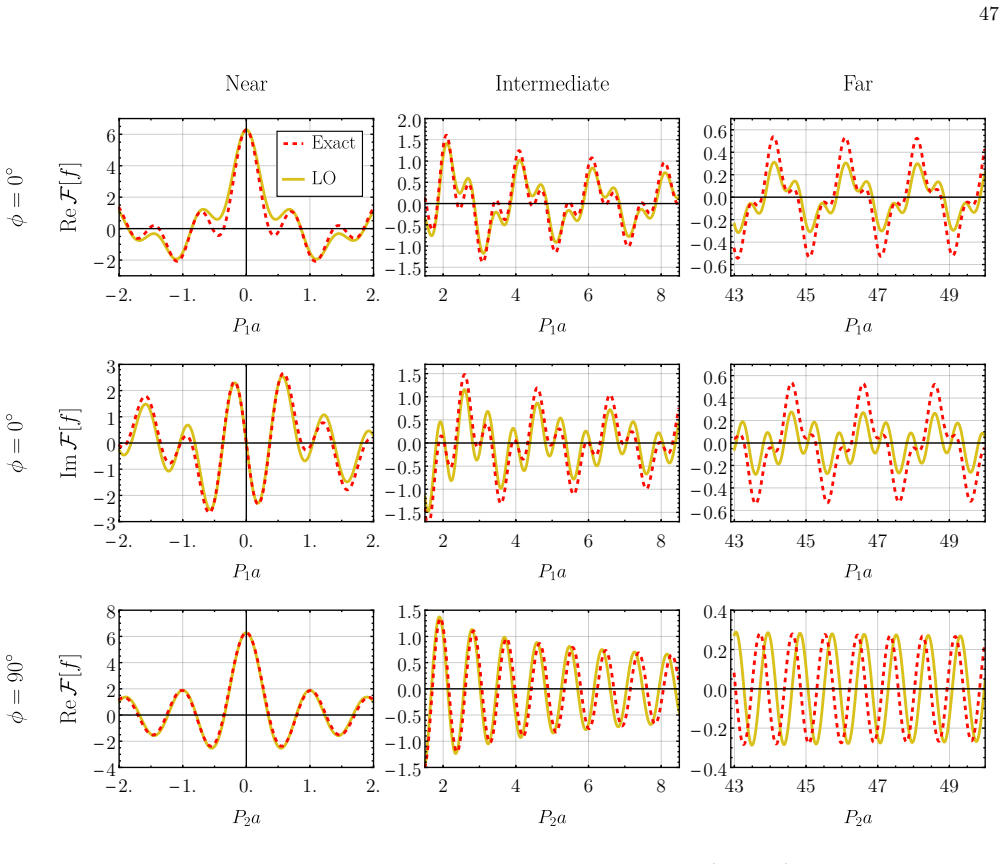
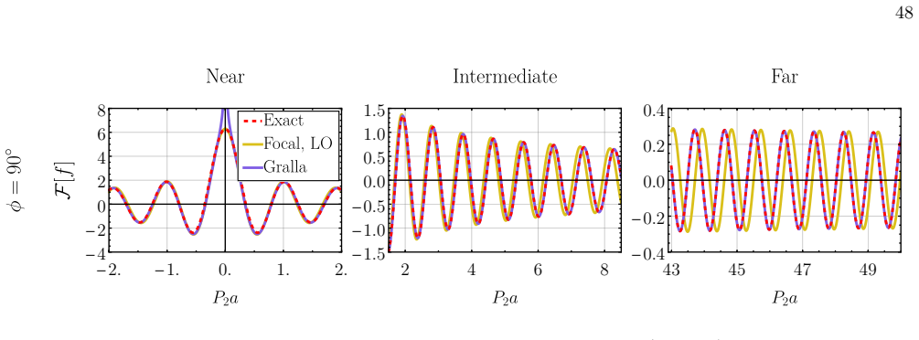
The authors derive a focal expansion that approximates the Hankel transforms arising in the Fourier transforms of radially symmetric or ring-like 2D functions. The leading term of this expansion provides a global approximation that is accurate at both small and large spatial frequencies for a wide class of such functions, as demonstrated through examples and application to toy models of photon rings.
What carries the argument
the focal expansion, a series approximation applied to the Hankel transforms of each angular mode that captures the transform behavior from low to high spatial frequencies in one expression
If this is right
- The method yields a single formula for interferometric visibilities of ring-like sources that works at both low and high baselines.
- It removes the need to switch between moment expansions at small frequencies and asymptotic forms at large frequencies.
- For photon-ring models it supplies the interferometric response directly, aiding analysis for missions targeting that feature.
- The approach applies to any 2D radially concentrated image without requiring separate low-frequency and high-frequency treatments.
Where Pith is reading between the lines
- The same style of expansion could be tested on 3D Fourier transforms or other oscillatory integrals that appear in wave propagation problems.
- Direct comparison against calibrated visibility data from existing or future arrays would show whether the approximation supports quantitative ring-radius measurements.
- Hybrid schemes that add the focal term to standard numerical integrators might extend the range to mildly non-ring images.
Load-bearing premise
The input images must be radially concentrated ring-like functions, and the leading focal term by itself must deliver sufficient accuracy without higher-order terms or per-case adjustments.
What would settle it
Numerically compute the exact 2D Fourier transform of a Gaussian ring profile or similar test function, then compare it to the leading focal term output over a dense grid of spatial frequencies from near zero to large values; persistent low relative error across the full range would support the claim.
Figures

read the original abstract
We derive and showcase a novel approach to approximating Fourier transforms in higher dimensions, focusing specifically on the case of 2D radially concentrated ('ring-like') functions. We first reduce the problem to that of evaluating the Hankel transforms of each angular mode of the image and then use our focal expansion to approximate these remaining Hankel transforms. Our method provides a single approximation that remains accurate from small to large spatial frequencies, bridging regimes where moment-based or large-frequency asymptotic expansions are individually reliable. We explore a series of examples, showing that the leading focal term provides an accurate global approximation for a broad range of functions. We demonstrate the utility of this approximation by examining the interferometric response for toy models of a black hole's "photon ring," highlighting the application to experiments designed to measure this feature such as the Black Hole Explorer.
Editorial analysis
A structured set of objections, weighed in public.
Referee Report
Summary. The paper derives a focal expansion to approximate the 2D Fourier transform of radially concentrated ('ring-like') functions. It reduces the problem to Hankel transforms of angular modes and approximates those transforms via the leading term of the focal expansion, claiming this single approximation remains accurate from small to large spatial frequencies and bridges moment-based and large-frequency asymptotic regimes. The utility is demonstrated on toy models of black hole photon rings for interferometric applications such as the Black Hole Explorer.
Significance. If the leading focal term can be shown to deliver controlled accuracy for general ring-like profiles, the method would offer a practical, unified tool for computing Fourier transforms in astrophysical imaging, especially for photon-ring modeling where efficient evaluation across frequency regimes is valuable. The reduction to Hankel transforms and the concrete interferometry examples are clear strengths; the absence of a general error bound currently limits the result's immediate applicability beyond the presented cases.
major comments (2)
- [focal expansion derivation and error analysis] The central claim that the leading focal term alone suffices for accurate global approximation of the Hankel transforms (and thus the 2D FT) for a broad range of radially concentrated functions lacks a derivation or bound on the truncation error. Without this, it is impossible to assess whether the approximation degrades for broader, multi-peaked, or otherwise non-ideal radial profiles outside the specific toy-model widths and contrasts shown.
- [examples and validation] Validation in the examples relies on a handful of photon-ring toy models with fixed radial parameters and frequency ranges. No systematic study (e.g., error metrics versus radial width, contrast, or number of peaks) is provided to support the assertion that the leading term works across a 'broad range' without case-by-case tuning or higher-order corrections.
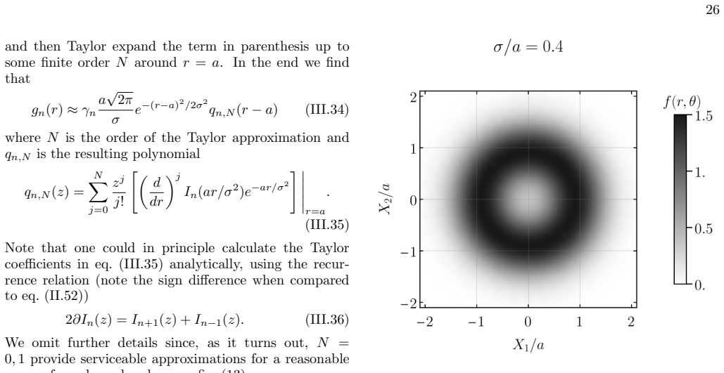
minor comments (2)
- [derivation sections] Ensure all equations for the focal expansion, its relation to the Hankel transform, and the angular-mode decomposition are explicitly stated with consistent notation.
- [figures and examples] Add a brief comparison table or plot quantifying the approximation error against standard moment expansions and asymptotic forms for the same test functions.
Simulated Author's Rebuttal
We thank the referee for the constructive and detailed report. The comments correctly identify that the manuscript relies primarily on examples rather than a general error bound, and that the validation could be more systematic. We address each point below and will incorporate revisions to strengthen the presentation of the focal expansion's accuracy and applicability.
read point-by-point responses
-
Referee: The central claim that the leading focal term alone suffices for accurate global approximation of the Hankel transforms (and thus the 2D FT) for a broad range of radially concentrated functions lacks a derivation or bound on the truncation error. Without this, it is impossible to assess whether the approximation degrades for broader, multi-peaked, or otherwise non-ideal radial profiles outside the specific toy-model widths and contrasts shown.
Authors: Section 2 derives the focal expansion and isolates the leading term for the Hankel transform of each angular mode. The manuscript does not supply a general truncation-error bound that holds for arbitrary radial profiles. We agree this omission makes it difficult to judge performance outside the demonstrated cases. In revision we will add a brief discussion of the leading-term error scaling with radial concentration (drawing on the expansion's asymptotic properties) together with numerical error estimates for the existing toy models and one additional broader-profile case. revision: partial
-
Referee: Validation in the examples relies on a handful of photon-ring toy models with fixed radial parameters and frequency ranges. No systematic study (e.g., error metrics versus radial width, contrast, or number of peaks) is provided to support the assertion that the leading term works across a 'broad range' without case-by-case tuning or higher-order corrections.
Authors: The examples in Section 3 use several photon-ring toy models with different radial widths and contrasts to illustrate global accuracy. We acknowledge that these do not constitute a systematic parameter survey. We will expand the validation to include quantitative error metrics (relative L2 and pointwise errors) plotted against radial width, contrast, and a two-peak configuration, all evaluated over the same frequency range used for the interferometric examples. revision: yes
Circularity Check
No circularity: focal expansion derived independently from Hankel reduction
full rationale
The paper reduces the 2D Fourier transform of radially concentrated functions to a set of Hankel transforms over angular modes, then introduces the focal expansion as a direct approximation for those transforms. This chain is presented as a mathematical derivation without any self-definition (the expansion is not defined using the target FT result), without fitting parameters to data and relabeling them as predictions, and without load-bearing self-citations or imported uniqueness theorems. Validation occurs via explicit examples on toy models rather than by construction, and the leading-term claim is tested rather than assumed tautologically. The derivation remains self-contained against external benchmarks.
Axiom & Free-Parameter Ledger
invented entities (1)
-
focal expansion
no independent evidence
Reference graph
Works this paper leans on
- [1]
- [2]
-
[3]
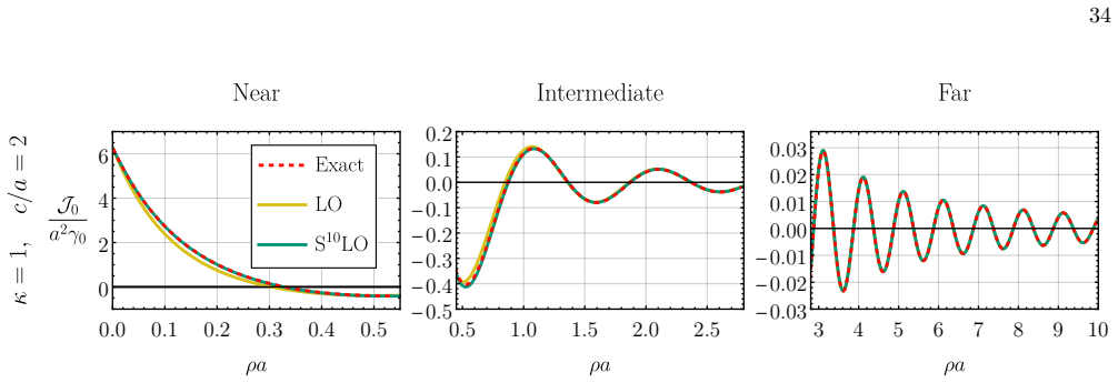
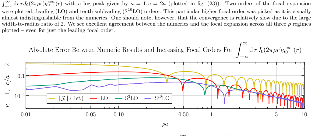
0 2 4 6 8 10 1 2 3 4 5 -0.2 -0.1 0.0 0.1 0.2 40 42 44 46 48 50 -6
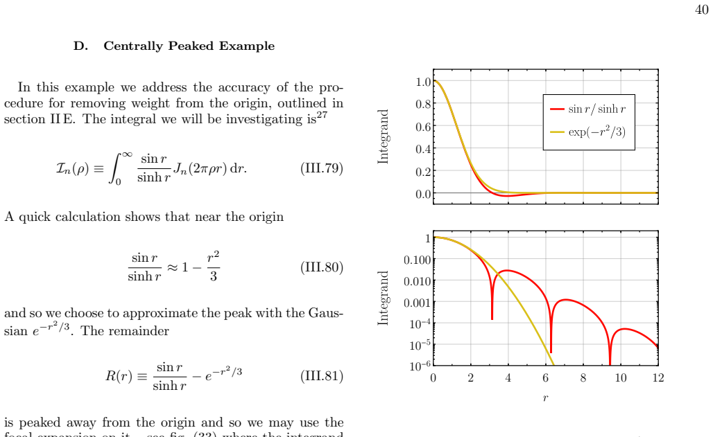
0.2 0.4 0.6 0.8 1. 0 2 4 6 8 10 1 2 3 4 5 -0.2 -0.1 0.0 0.1 0.2 40 42 44 46 48 50 -6. × 10-4 -3. × 10-4 0
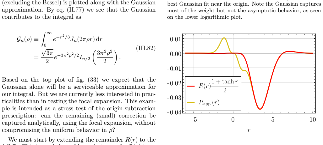
-
[4]
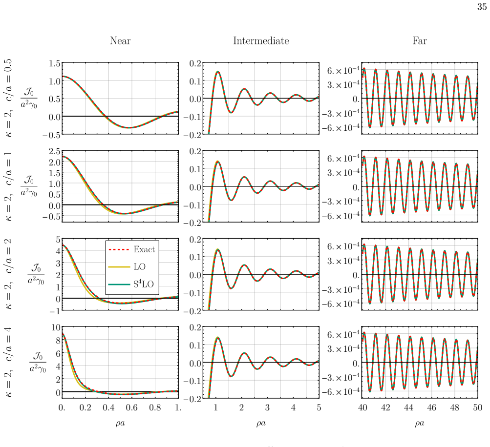
× 10-4 FIG. 26. Comparison of the numerical evaluation (dashed red) of R ∞ −∞ dr rJ0(2πρr)g ext. 0 (r) for a log peak withκ= 2 and several values ofcto the focal expansion at LO (yellow) and S 4LO (green). We see excellent agreement across all plots, with notable errors only visible around the origin for the LO at large width values. The fourth subleading...
-
[5]
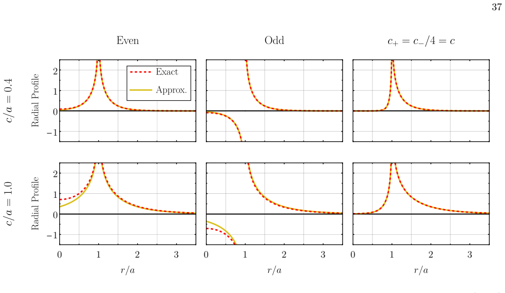
K0 2e−γE r−a c +K 0 2e−γE r+a c # (III.65) f o(c)(r, θ) =γ(θ)
Example 2: Asymmetric Divergence We now move to a different extension of the logarith- mic divergence eq. (III.45). We denote byK 0 the mod- ified Bessel function of the second kind of order zero. One can show that the following hold (assumingz >0 is a positive real number) [15] K0(z) z≪1 ≈log 2e−γE z ,(III.62) K0(z) z≫1 ≈ r π 2z e−z,(III.63) withγ E ≈0.5...
-
[6]
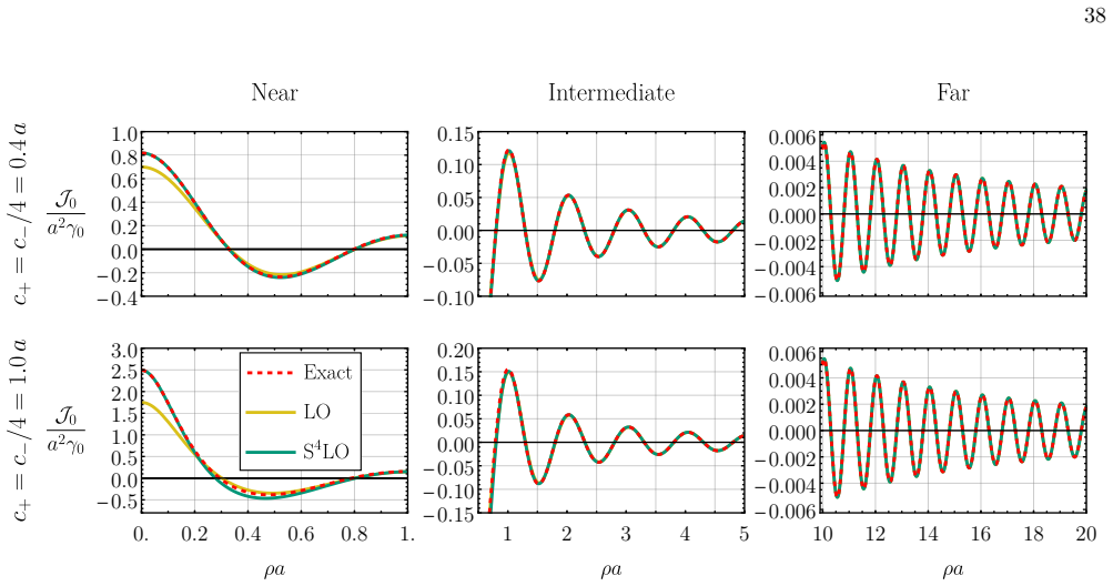
0.2 0.4 0.6 0.8 1. -0.5 0.0 0.5 1.0 1.5 2.0 2.5 3.0 1 2 3 4 5 -0.15 -0.10 -0.05 0.00 0.05 0.10 0.15 0.20 10 12 14 16 18 20 -0.006 -0.004 -0.002 0.000 0.002 0.004 0.006 FIG. 29. Comparison of the numeric (dashed red) and focal (yellow, green) results forJ 0 in the case of two mixedK 0 peaks withc + =c −/4 for two values ofc +. We see the focal LO eq. (III....
-
[7]
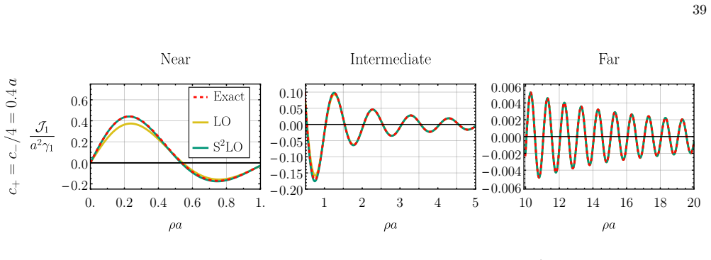
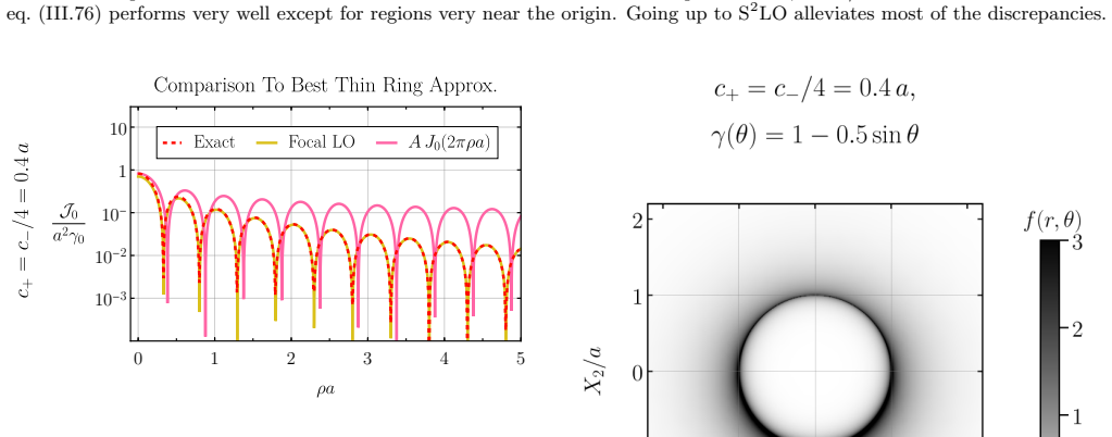
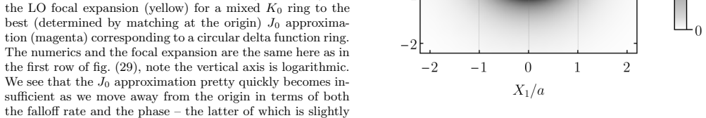
0.2 0.4 0.6 0.8 1. -0.2 0.0 0.2 0.4 0.6 1 2 3 4 5 -0.20 -0.15 -0.10 -0.05 0.00 0.05 0.10 10 12 14 16 18 20 -0.006 -0.004 -0.002 0.000 0.002 0.004 0.006 FIG. 30. Comparison of the numeric results forJ 1 in the case of a mixedK 0 peak withc + =c −/4 = 0.4. We see the focal LO eq. (III.76) performs very well except for regions very near the origin. Going up ...
-
[8]
General Calculations For our final set of examples we analyze the case of rings of zero thickness – those whose radial profile is a Dirac delta. We specialize to curves whose radial distance from the origin can be written as a positive function of 28 What makes us suspect this second comment might be true is that the subleading focal orders help insomepla...
-
[9]
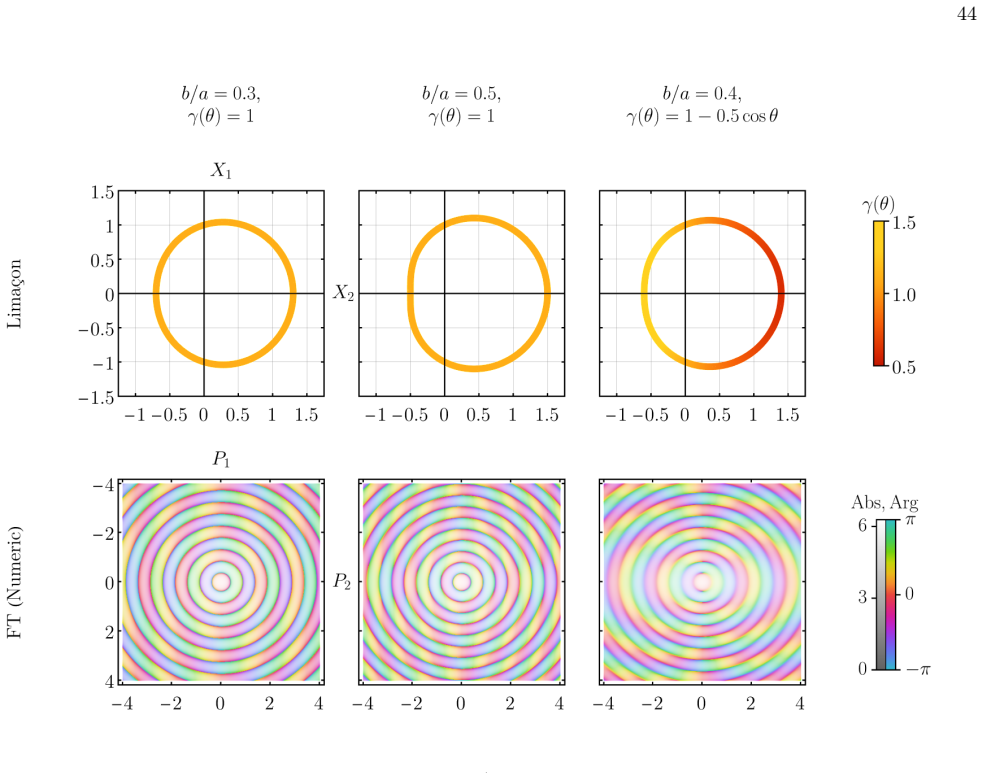
The Lima¸ con The lima¸ con is the curve given by R(θ) =a+bcos(θ+δ) (III.99) wherea, b, δare real constants. We assumea >0 and a/b >1, the latter condition coming from requiring the lima¸ con to be a smooth, non-self-intersecting curve [25]. This family of curves corresponds arguably to the sim- plest functionR(θ) one can write down (beaten only by the ci...
-
[10]
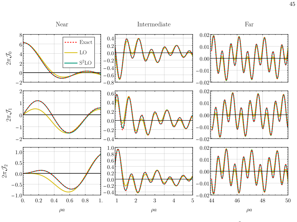
0.2 0.4 0.6 0.8 1. -1.0 -0.5 0.0 0.5 1.0 1 2 3 4 5 -0.4 -0.2 0.0 0.2 0.4 0.6 0.8 1.0 44 46 48 50 -0.02 -0.01 0.00 0.01 0.02 FIG. 38. Comparisons of the numerical evaluations of the integralsJ 0,J 1, andJ 2 to the LO and S 2LO focal expansion for the middle lima¸ con of fig. (37) withb/a= 0.5. The LO provides a serviceable and the S 2LO an excellent approx...
-
[11]
0.1 0.2 0.3 0.4 0.5 0.6 -1.0 -0.5 0.0 0.5 1.0
-
[12]
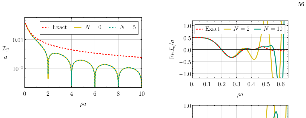
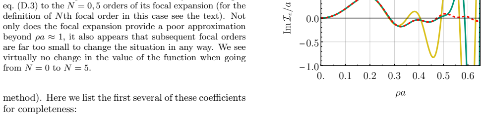
0.1 0.2 0.3 0.4 0.5 0.6 -1.0 -0.5 0.0 0.5 1.0 FIG. 44. Comparison of the real and imaginary parts of the exact oscillatory integral eq. (D.6) to itsN= 2,10 order focal approximations (for the definition ofNth order in this case see the text). We see that, unlike in fig. (43), successive fo- cal orders do appear to significantly improve the performance of ...
-
[13]
R. N. Bracewell,The Fourier transform and its applica- tions, 3rd ed., McGraw-Hill series in electrical and com- puter engineering. Circuits and systems (McGraw Hill, Boston, 2000)
work page 2000
-
[14]
B. Osgood,Lectures on the Fourier transform and its applications, Sally series (Providence, R.I.) (American Mathematical Society, Providence, Rhode Island, 2019)
work page 2019
-
[15]
E. M. Stein,Fourier analysis : an introduction, Prince- ton lectures in analysis 1 (Princeton University Press, Princeton, N.J., 2003)
work page 2003
-
[16]
The Event Horizon Telescope Collaborationet all, First m87 event horizon telescope results. i. the shadow of the supermassive black hole, The Astrophysical Journal Let- ters875, L1 (2019)
work page 2019
-
[17]
Event Horizon Telescope Collaborationet all, First sagit- tarius a* event horizon telescope results. i. the shadow of the supermassive black hole in the center of the milky way, The Astrophysical Journal Letters930, L12 (2022)
work page 2022
-
[18]
J. M. Bardeen, Timelike and null geodesics in the Kerr metric., inBlack Holes (Les Astres Occlus)(1973) pp. 215–239
work page 1973
-
[19]
J. P. Luminet, Image of a spherical black hole with thin accretion disk., Astronomy and Astrophysics75, 228 (1979)
work page 1979
-
[20]
S. E. Gralla, D. E. Holz, and R. M. Wald, Black hole shadows, photon rings, and lensing rings, Phys. Rev. D 100, 024018 (2019)
work page 2019
-
[21]
M. D. Johnson, A. Lupsasca, A. Strominger, G. N. Wong, S. Hadar, D. Kapec, R. Narayan, A. Chael, C. F. Gammie, P. Galison, D. C. M. Palumbo, S. S. Doeleman, L. Blackburn, M. Wielgus, D. W. Pesce, J. R. Farah, and J. M. Moran, Universal interferometric signatures of a black hole’s pho- ton ring, Science Advances6, eaaz1310 (2020), https://www.science.org/d...
-
[22]
M. D. Johnson, K. Akiyama, R. Baturin, B. Bi- lyeu, L. Blackburn, D. Boroson, A. C´ ardenas-Avenda˜ no, A. Chael, C.-k. Chan, D. Chang, P. Cheimets, C. Chou, S. S. Doeleman, J. Farah, P. Galison, R. Gamble, C. F. Gammie, Z. Gelles, J. L. G´ omez, S. E. Gralla, P. Grimes, L. I. Gurvits, S. Hadar, K. Haworth, K. Hada, M. H. Hecht, M. Honma, J. Houston, B. H...
-
[23]
A. R. Thompson, J. M. Moran, and J. Swenson, 58 George W.,Interferometry and Synthesis in Radio As- tronomy, 3rd Edition(2017)
work page 2017
-
[24]
S. E. Gralla, Measuring the shape of a black hole photon ring, Phys. Rev. D102, 044017 (2020)
work page 2020
-
[25]
H. Jia, E. Quataert, A. Lupsasca, and G. N. Wong, Pho- ton ring interferometric signatures beyond the universal regime, Phys. Rev. D110, 083044 (2024)
work page 2024
- [26]
-
[27]
G. Watson,A Treatise on the Theory of Bessel Functions, Cambridge Mathematical Library (Cambridge University Press, 1995)
work page 1995
-
[28]
C. Bender and S. Orszag,Advanced Mathematical Meth- ods for Scientists and Engineers: Asymptotic Methods and Perturbation Theory, Vol. 1 (Springer New York, 1999)
work page 1999
- [29]
-
[30]
H. Bateman and B. M. Project,Tables of Integral Trans- forms(McGraw-Hill Book Company, 1954)
work page 1954
-
[31]
M. Abramowitz and I. Stegun,Handbook of Mathematical Functions: With Formulas, Graphs, and Mathematical Tables, Applied mathematics series (Dover Publications, 1965)
work page 1965
-
[32]
R. Beals and J. Szmigielski, Meijer G-functions: a gen- tle introduction, Notices of the American Mathematical Society60, 866 (2013)
work page 2013
-
[33]
Luke,The Special Functions and Their Approxima- tions, Mathematics in science and engineering No
Y. Luke,The Special Functions and Their Approxima- tions, Mathematics in science and engineering No. v. 1 (Academic Press, 1969)
work page 1969
-
[34]
J. L. Fields, The asymptotic expansion of the meijer g- function, Mathematics of Computation26, 757 (1972)
work page 1972
-
[35]
P. Kuklinski and D. A. Hague, Identities and properties of multi-dimensional generalized bessel functions (2021), arXiv:1908.11683 [math.GM]
-
[36]
S. Lorenzutta, G. Maino, G. Dattoli, A. Torre, and C. Chiccoli, Infinite-variable bessel functions of the anger type and the fourier expansions, Reports on Mathemati- cal Physics39, 163–176 (1997)
work page 1997
-
[37]
J. T. Grossman and M. P. Grossman, Dimple or no dim- ple, The Two-Year College Mathematics Journal13, 52 (1982)
work page 1982
-
[38]
J. R. Farah, D. W. Pesce, M. D. Johnson, and L. Black- burn, On the approximation of the black hole shadow with a simple polar curve, The Astrophysical Journal 900, 77 (2020)
work page 2020
-
[39]
The Black Hole Explorer: photon ring science, detection, and shape measurement,
A. Lupsasca, A. C´ ardenas-Avenda˜ no, D. C. M. Palumbo, M. D. Johnson, S. E. Gralla, D. P. Marrone, P. Gali- son, P. Tiede, and L. Keeble, The Black Hole Explorer: photon ring science, detection, and shape measurement, inSpace Telescopes and Instrumentation 2024: Opti- cal, Infrared, and Millimeter Wave, Society of Photo- Optical Instrumentation Engineer...
-
[40]
C. Efthimiou and C. Frye,Spherical Harmonics in p Di- mensions(World Scientific, 2014)
work page 2014
-
[41]
R. Bapat and E. Ghorbani, Inverses of triangular matri- ces and bipartite graphs, Linear Algebra and its Appli- cations447, 68 (2014)
work page 2014
discussion (0)
Sign in with ORCID, Apple, or X to comment. Anyone can read and Pith papers without signing in.