State and Trajectory Estimation of Tensegrity Robots via Factor Graphs and Chebyshev Polynomials
Pith reviewed 2026-05-10 17:01 UTC · model grok-4.3
The pith
Factor graphs fused with Chebyshev polynomials yield continuous-time state and trajectory estimates for tensegrity robots by combining RGB-D camera and cable length data.
A machine-rendered reading of the paper's core claim, the machinery that carries it, and where it could break.
Core claim
The authors claim that a factor-graph formulation, augmented by Mahalanobis-distance clustering for noise handling and Chebyshev polynomial interpolation for velocity estimation, produces high-fidelity continuous-time estimates of every rigid link on a tensegrity robot and outperforms an ICP baseline on both simulated and real data.
What carries the argument
Factor graphs that encode the robot's structural connectivity for multi-sensor fusion, paired with Chebyshev polynomials that fit smooth trajectories and velocities between discrete measurements.
If this is right
- Closed-loop controllers can use the continuous state stream for real-time feedback instead of waiting for discrete updates.
- System identification routines gain denser, smoother data for learning the robot's compliance parameters.
- Machine-learning policies trained on the estimated trajectories inherit higher fidelity than those trained on ICP outputs.
- The same graph structure can be reused for both online filtering and offline smoothing without redesign.
- Outlier rejection via Mahalanobis clustering remains effective even when one sensor modality degrades.
Where Pith is reading between the lines
- The same factor-graph template could be adapted to other cable-driven or soft robots that combine vision with internal length or tension sensors.
- Replacing Chebyshev polynomials with learned basis functions might further reduce error on highly non-polynomial motions.
- Extending the graph to include learned dynamics factors could close the loop between estimation and control in a single optimization.
- Testing on larger or reconfigurable tensegrity structures would reveal whether the current sensor suite scales without additional cameras.
Load-bearing premise
That RGB-D images and cable-length readings can be fused through factor graphs in a way that consistently overcomes the robot's nonlinear and underconstrained dynamics without extra motion constraints.
What would settle it
A set of real-robot trials in which the estimated bar trajectories diverge by more than a few centimeters from synchronized motion-capture ground truth during fast, multi-bar folding maneuvers would falsify the accuracy claims.
Figures


read the original abstract
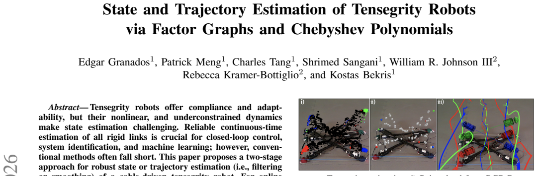
Tensegrity robots offer compliance and adaptability, but their nonlinear, and underconstrained dynamics make state estimation challenging. Reliable continuous-time estimation of all rigid links is crucial for closed-loop control, system identification, and machine learning; however, conventional methods often fall short. This paper proposes a two-stage approach for robust state or trajectory estimation (i.e., filtering or smoothing) of a cable-driven tensegrity robot. For online state estimation, this work introduces a factor-graph-based method, which fuses measurements from an RGB-D camera with on-board cable length sensors. To the best of the authors' knowledge, this is the first application of factor graphs in this domain. Factor graphs are a natural choice, as they exploit the robot's structural properties and provide effective sensor fusion solutions capable of handling nonlinearities in practice. Both the Mahalanobis distance-based clustering algorithm, used to handle noise, and the Chebyshev polynomial method, used to estimate the most probable velocities and intermediate states, are shown to perform well on simulated and real-world data, compared to an ICP-based algorithm. Results show that the approach provides high fidelity, continuous-time state and trajectory estimates for complex tensegrity robot motions.
Editorial analysis
A structured set of objections, weighed in public.
Referee Report
Summary. The paper proposes a two-stage pipeline for state and trajectory estimation of cable-driven tensegrity robots. The first stage uses factor graphs to fuse RGB-D camera data with onboard cable-length sensors, incorporating Mahalanobis-distance clustering to manage noise and exploiting the robot's structural properties for nonlinear sensor fusion. The second stage fits Chebyshev polynomials to the factor-graph output to recover continuous-time velocities and intermediate states. The method is presented as the first application of factor graphs to this domain and is claimed to deliver high-fidelity estimates that outperform ICP on both simulated and real data.
Significance. If the physical consistency of the continuous-time trajectories can be guaranteed, the work would provide a practical advance for compliant, underconstrained robots where reliable state estimation is a prerequisite for closed-loop control and learning. The explicit use of factor graphs to encode structural constraints is a natural and potentially reusable modeling choice, and the addition of Chebyshev smoothing addresses the need for dense, differentiable trajectories.
major comments (2)
- [Chebyshev polynomial method / trajectory estimation] In the section describing the Chebyshev polynomial stage (following the factor-graph optimization), the polynomials are fitted independently to produce velocities and intermediate states. No mechanism is described for projecting the resulting continuous trajectory back onto the manifold of rigid bar lengths and fixed cable lengths that were enforced in the factor-graph solution. Without such a projection or joint optimization, small fitting errors can produce kinematically inconsistent trajectories, which is especially problematic for the underconstrained tensegrity dynamics emphasized in the introduction.
- [Results / evaluation] The results section asserts superior performance over ICP on simulated and real data, yet the abstract and summary provide no numerical error metrics (e.g., RMSE on pose or velocity, success rates, or statistical comparisons). Without these quantitative values and details on how nonlinearities and under-constrained modes are handled, the central claim of “high fidelity” remains difficult to evaluate.
minor comments (2)
- [Abstract] The abstract would benefit from at least one concrete performance number (e.g., average position error reduction versus ICP) to support the claim of superiority.
- [Notation / preliminaries] Notation for robot states, cable lengths, and polynomial coefficients should be introduced once and used consistently; a short table of symbols would improve readability.
Simulated Author's Rebuttal
We thank the referee for the constructive feedback, which highlights important aspects of physical consistency and quantitative evaluation. We address each major comment below and will incorporate revisions to strengthen the manuscript.
read point-by-point responses
-
Referee: In the section describing the Chebyshev polynomial stage (following the factor-graph optimization), the polynomials are fitted independently to produce velocities and intermediate states. No mechanism is described for projecting the resulting continuous trajectory back onto the manifold of rigid bar lengths and fixed cable lengths that were enforced in the factor-graph solution. Without such a projection or joint optimization, small fitting errors can produce kinematically inconsistent trajectories, which is especially problematic for the underconstrained tensegrity dynamics emphasized in the introduction.
Authors: We agree that ensuring kinematic consistency is critical for underconstrained tensegrity systems. The factor-graph optimization explicitly enforces rigid-bar and cable-length constraints at the discrete states via dedicated factors. The subsequent Chebyshev fitting approximates these states and derives velocities in a least-squares sense, with our experiments indicating that deviations remain small. However, to provide an explicit guarantee, we will add a post-processing projection step in the revised manuscript. This step will solve a constrained optimization problem to adjust the polynomial coefficients minimally while restoring satisfaction of the length constraints, and we will report its effect on trajectory fidelity. revision: yes
-
Referee: The results section asserts superior performance over ICP on simulated and real data, yet the abstract and summary provide no numerical error metrics (e.g., RMSE on pose or velocity, success rates, or statistical comparisons). Without these quantitative values and details on how nonlinearities and under-constrained modes are handled, the central claim of “high fidelity” remains difficult to evaluate.
Authors: The full results section of the manuscript already presents quantitative metrics, including RMSE values for pose and velocity estimates, trajectory fitting errors, and direct comparisons against ICP on both simulated and real data, along with discussion of the factor-graph handling of nonlinearities and under-constrained modes through structural factors. We acknowledge that these details are not summarized in the abstract. In the revision we will update the abstract and summary to include key numerical results (e.g., average RMSE reductions and success rates) and a concise statement on the treatment of nonlinearities. revision: yes
Circularity Check
No significant circularity; derivation relies on standard sensor fusion and polynomial approximation.
full rationale
The paper presents a two-stage pipeline using factor graphs to fuse RGB-D and cable-length measurements followed by Chebyshev polynomial fitting for continuous-time velocities and states. No equations or steps reduce the claimed estimates to fitted parameters by construction, nor do they depend on self-citations for uniqueness or load-bearing premises. The approach is benchmarked against ICP on simulated and real data, with the central claims resting on empirical performance rather than tautological definitions or renamed inputs. This is a standard application of existing techniques without self-referential reduction.
Axiom & Free-Parameter Ledger
axioms (1)
- domain assumption Factor graphs can effectively exploit the structural properties of tensegrity robots and handle their nonlinearities in practice
Reference graph
Works this paper leans on
-
[1]
Factor graphs for robot perception,
F. Dellaert, M. Kaess,et al., “Factor graphs for robot perception,” F oundations and Trends® in Robotics, 2017
work page 2017
-
[2]
E. Granados, S. Tangirala, and K. E. Bekris, “Kinodynamic trajec- tory following with stela: Simultaneous trajectory estimation & local adaptation,”RSS, 2025
work page 2025
-
[3]
Continuous-time state & dynamics estimation using a pseudo-spectral parameterization,
V . Agrawal and F. Dellaert, “Continuous-time state & dynamics estimation using a pseudo-spectral parameterization,” in2021 ICRA
-
[4]
6n-dof pose tracking for tensegrity robots,
S. Lu, W. R. Johnson III, K. Wang, X. Huang, J. Booth, R. Kramer- Bottiglio, and K. Bekris, “6n-dof pose tracking for tensegrity robots,” inISRR. Springer, 2022
work page 2022
-
[5]
Real2sim2real transfer for control of cable-driven robots via a differentiable physics engine,
K. Wang, W. R. Johnson, S. Lu, X. Huang, J. Booth, R. Kramer- Bottiglio, M. Aanjaneya, and K. Bekris, “Real2sim2real transfer for control of cable-driven robots via a differentiable physics engine,” in IROS. IEEE, 2023, pp. 2534–2541
work page 2023
-
[6]
On-manifold preintegration for real-time visual–inertial odometry,
C. Forster, L. Carlone, F. Dellaert, and D. Scaramuzza, “On-manifold preintegration for real-time visual–inertial odometry,”IEEE Transac- tions on Robotics, vol. 33, no. 1, pp. 1–21, 2016
work page 2016
-
[7]
Continuous-time state estimation methods in robotics: A survey,
W. Talbot, J. Nubert, T. Tuna, C. Cadena, F. D ¨umbgen, J. Tordesillas, T. D. Barfoot, and M. Hutter, “Continuous-time state estimation methods in robotics: A survey,”IEEE Transactions on Robotics, 2025
work page 2025
-
[8]
D. S. Shah, J. W. Booth, R. L. Baines, K. Wang, M. Vespig- nani, K. Bekris, and R. Kramer-Bottiglio, “Tensegrity robotics,”Soft robotics, vol. 9, no. 4, pp. 639–656, 2022
work page 2022
-
[9]
Design of superball v2, a compliant tensegrity robot for absorbing large impacts,
M. Vespignani, J. M. Friesen, V . SunSpiral, and J. Bruce, “Design of superball v2, a compliant tensegrity robot for absorbing large impacts,” inIROS, 2018, pp. 2865–2871
work page 2018
-
[10]
Adaptive and resilient soft tensegrity robots,
J. Rieffel and J.-B. Mouret, “Adaptive and resilient soft tensegrity robots,”Soft robotics, vol. 5, no. 3, pp. 318–329, 2018
work page 2018
-
[11]
P. Meng, W. Wang, D. Balkcom, and K. E. Bekris,Proof-of-Concept Designs for the Assembly of Modular Dynamic Tensegrities into Easily Deployable Structures. Earth and Space, 2021
work page 2021
-
[12]
Tensegrity robot proprioceptive state estimation with geometric con- straints,
W. Tong, T.-Y . Lin, J. Mi, Y . Jiang, M. Ghaffari, and X. Huang, “Tensegrity robot proprioceptive state estimation with geometric con- straints,”IEEE Robotics and Automation Letters, 2025
work page 2025
-
[13]
Learning differentiable tensegrity dynamics using graph neural networks,
N. Chen, K. Wang, W. R. Johnson III, R. Kramer-Bottiglio, K. Bekris, and M. Aanjaneya, “Learning differentiable tensegrity dynamics using graph neural networks,”arXiv preprint arXiv:2410.12216, 2024
-
[14]
An open- source, reproducible tensegrity robot that can navigate among obstacles,
W. R. J. III, P. Meng, N. Chen, L. Cimatti, A. Vercoutere, M. Aanjaneya, R. Kramer-Bottiglio, and K. E. Bekris, “An open- source, reproducible tensegrity robot that can navigate among obstacles,” 2025. [Online]. Available: https://arxiv.org/abs/2511.05798
-
[15]
A micro lie theory for state estimation in robotics,
J. Sola, J. Deray, and D. Atchuthan, “A micro lie theory for state estimation in robotics,”arXiv preprint arXiv:1812.01537, 2018
-
[16]
L. N. Trefethen,Approximation theory and approximation practice, extended edition. SIAM, 2019
work page 2019
-
[17]
Barycentric lagrange interpolation,
J.-P. Berrut and L. N. Trefethen, “Barycentric lagrange interpolation,” SIAM review, vol. 46, no. 3, pp. 501–517, 2004
work page 2004
-
[18]
On the generalised distance in statistics. sankhya a, 80 (suppl 1), 1–7 (2018),
P. Mahalanobis, “On the generalised distance in statistics. sankhya a, 80 (suppl 1), 1–7 (2018),” 1936
work page 2018
-
[19]
B. F. Manly, J. A. N. Alberto, and K. Gerow,Multivariate statistical methods: a primer. Chapman and Hall/CRC, 2024
work page 2024
-
[20]
Mahalanobis distances and ecological niche mod- elling: correcting a chi-squared probability error,
T. R. Etherington, “Mahalanobis distances and ecological niche mod- elling: correcting a chi-squared probability error,” 2019
work page 2019
-
[21]
Imu preinte- gration on manifold for efficient visual-inertial maximum-a-posteriori estimation,
C. Forster, L. Carlone, F. Dellaert, and D. Scaramuzza, “Imu preinte- gration on manifold for efficient visual-inertial maximum-a-posteriori estimation,” 2015
work page 2015
-
[22]
J. L. Aurentz and L. N. Trefethen, “Chopping a chebyshev series,” ACM Transactions on Mathematical Software (TOMS), 2017
work page 2017
discussion (0)
Sign in with ORCID, Apple, or X to comment. Anyone can read and Pith papers without signing in.