Towards Optimal Passive Feedback Control of LTI Systems under LQR Performance

Armin Gie{\ss}ler; Pol Jan\'e-Soneira; S\"oren Hohmann

arxiv: 2604.14854 · v2 · submitted 2026-04-16 · 🧮 math.OC · cs.SY· eess.SY

Towards Optimal Passive Feedback Control of LTI Systems under LQR Performance

Armin Gie{\ss}ler , Pol Jan\'e-Soneira , S\"oren Hohmann This is my paper

Pith reviewed 2026-05-10 11:05 UTC · model grok-4.3

classification 🧮 math.OC cs.SYeess.SY MSC 93C0593B5249M37

keywords passive feedbackLTI systemsLQR performancestate-feedback designbilinear matrix inequalitiesprojected gradient flowpolytope approximation

0 comments

The pith

Feedback gains for LTI systems can be chosen to ensure passivity while minimizing LQR cost by inner-approximating the passivating set with a convex polytope and running projected gradient flow inside it.

A machine-rendered reading of the paper's core claim, the machinery that carries it, and where it could break.

The paper addresses the problem of designing state feedback for continuous-time linear time-invariant systems so that the closed-loop system is passive with respect to an external input-output port and the LQR cost is minimized when disturbances are absent. Direct optimization is blocked by bilinear matrix inequalities, so the authors first characterize the set of all passivating gains as unbounded, possibly nonconvex, path-connected and contractible. They then replace this set with a compact convex polytope that lies inside it and apply a projected gradient flow to locate the point inside the polytope that yields the smallest LQR cost. Numerical examples confirm that the resulting gains produce closed-loop passivity and competitive performance.

Core claim

The set of passivating feedback gains is unbounded, possibly nonconvex, path-connected and contractible; this set can be inner-approximated by a compact convex polytope inside which a projected gradient flow finds a gain that minimizes the LQR cost.

What carries the argument

Inner approximation of the passivating-gain set by a compact convex polytope, followed by projected gradient flow to minimize the LQR cost inside the polytope.

If this is right

Passivity constraints can be handled indirectly without solving the original bilinear matrix inequalities.
The projected gradient flow stays inside the polytope and therefore produces a gain that is guaranteed to be passivating.
The method applies to any LTI system for which a suitable inner polytope can be constructed from the passivity LMI.
Numerical examples demonstrate that the computed gains achieve closed-loop passivity together with low LQR cost.

Where Pith is reading between the lines

These are editorial extensions of the paper, not claims the author makes directly.

The same polytope-plus-gradient approach could be tried with other convex performance indices besides LQR, provided the index remains convex on the polytope.
If the polytope is chosen adaptively rather than fixed in advance, the gap between the approximated and true optimum might be reduced without losing convexity.
The contractibility of the true passivating set suggests that homotopy methods could be used to enlarge the polytope on the fly while preserving feasibility.

Load-bearing premise

A compact convex polytope can be chosen that lies entirely inside the possibly nonconvex set of passivating gains and still contains a point whose LQR cost is close to the global minimum.

What would settle it

A concrete LTI system and external port for which every gain inside the chosen polytope either fails to render the closed loop passive or produces an LQR cost more than 20 percent higher than the lowest cost achievable by any passivating gain.

Figures

Figures reproduced from arXiv: 2604.14854 by Armin Gie{\ss}ler, Pol Jan\'e-Soneira, S\"oren Hohmann.

**Figure 2.** Figure 2: Overview of the three steps of the indirect approach [PITH_FULL_IMAGE:figures/full_fig_p005_2.png] view at source ↗

**Figure 3.** Figure 3: Illustration of the stability region K, the passivity region P, the verified cubes Ci , and their union PU . for all K ∈ vert(C), then every K ∈ C (strictly) passivates the system (25) with the common storage function S(x) = 1 2 x ⊤P x. Consequently C ⊆ P(+) . Proof: Let vert(C) = {K0 , . . . , Kr}. Every K ∈ C is a convex combination K = Pr i=1 λiKi P with λi ≥ 0 and r i λi = 1. Consider first the case D … view at source ↗

**Figure 5.** Figure 5: Structured overview of the logical dependencies of [PITH_FULL_IMAGE:figures/full_fig_p007_5.png] view at source ↗

**Figure 6.** Figure 6: Visualization of stability region K, the passivity region P, the verified cubes Ci , the convex inner approximation PC , the cost function fK − fK∗ and the trajectory of the projected gradient flow K(t). -6 -4 -2 0 K1 -2 0 2 4 6 K2 K P Ci PC fK ! fK$ K$ K(t) K^ K(0) 100 102 [PITH_FULL_IMAGE:figures/full_fig_p008_6.png] view at source ↗

**Figure 7.** Figure 7: Visualization analogous to Fig. 6, with cubes [PITH_FULL_IMAGE:figures/full_fig_p008_7.png] view at source ↗

read the original abstract

We study state-feedback design for continuous-time LTI systems with a control input and an external input-output pair. Our objective is to determine feedback gains that render the closed-loop system (strictly) passive with respect to the external port while minimizing the standard LQR cost in the disturbance-free case. The resulting constrained optimization problem is intractable due to bilinear matrix inequalities. We analyze the set of passivating gains, showing it is unbounded, possibly nonconvex, path-connected, and contractible. We propose an indirect approach, in which the set of passivating feedback gains is inner-approximated by a compact, convex polytope. A projected gradient flow is employed to compute a gain within this polytope that minimizes the LQR cost. Numerical examples illustrate the effectiveness of the method.

Editorial analysis

A structured set of objections, weighed in public.

Desk editor's note, referee report, simulated authors' rebuttal, and a circularity audit. Tearing a paper down is the easy half of reading it; the pith above is the substance, this is the friction.

Desk Editor's Note private letter to a colleague

The paper characterizes the set of passivating gains geometrically and offers a polytope inner-approximation plus projected gradient flow as a workable way to minimize LQR cost inside it, but without suboptimality bounds the result remains an unquantified compromise.

read the letter

The one or two things to know are that the authors characterize the set of state-feedback gains that make an LTI system passive and then approximate that set from inside by a convex polytope so they can run a projected gradient flow to minimize the LQR cost. This sidesteps the bilinear matrix inequalities that make the joint problem hard. The geometric properties they establish for the passivating gain set—unbounded, possibly nonconvex, yet path-connected and contractible—are useful and appear fresh in this combination. The indirect method of polytope inner-approximation followed by projected gradient descent on the standard LQR objective is a pragmatic engineering move when exact solutions are intractable. The numerical examples show that the procedure can find gains that satisfy passivity while keeping the LQR cost reasonable, which is the practical point. The main limitation is that the approximation is not accompanied by any guarantee on how far the obtained cost is from the true minimum over all passivating gains. Since the set can be nonconvex, the polytope leaves out feasible points, and without a bound on the suboptimality gap it is difficult to judge how good the result really is. Inside the polytope the LQR cost is still non-convex in the gain, so the flow converges only to a stationary point; nothing rules out better points inside the same polytope. The construction of the polytope itself is not detailed enough in the abstract to see how tight it can be made in general. These issues are inherent to the indirect approach but mean the method is more of a heuristic than a certified solution. This work is aimed at control theorists and engineers who need to enforce passivity constraints alongside quadratic performance in state-feedback design. Readers who already use LMI or passivity tools and want a way to optimize further will find the geometric view and the algorithmic template worth looking at. It is solid enough on the analysis side to merit a serious referee, even though the optimization guarantees are limited. I would send it to peer review so the details of the polytope construction and any numerical validation can be examined properly.

Referee Report

2 major / 2 minor

Summary. The manuscript studies state-feedback design for continuous-time LTI systems to render the closed-loop system (strictly) passive w.r.t. an external I/O port while minimizing the standard LQR cost in the disturbance-free case. It establishes that the set of passivating gains is unbounded, possibly nonconvex, path-connected, and contractible. Because the direct formulation leads to intractable bilinear matrix inequalities, the authors propose an indirect method that inner-approximates the passivating set by a compact convex polytope and applies projected gradient flow to minimize the LQR cost inside this polytope. Numerical examples are provided to illustrate the procedure.

Significance. If the polytope can be chosen so that its LQR-optimal point remains close to the true constrained optimum and the flow reliably locates a high-quality stationary point, the method supplies a practical computational route for jointly enforcing passivity and LQR performance. The geometric characterization of the passivating gain set (unboundedness, path-connectedness, contractibility) is a clear contribution to the literature on passivity constraints. The explicit algorithmic construction via projected gradient flow on a convex set is concrete and reproducible from the description.

major comments (2)

[Abstract / indirect approach] Abstract and the description of the indirect approach: the set of passivating gains is shown to be possibly nonconvex, so any compact convex polytope necessarily excludes feasible gains. No explicit construction of the polytope (e.g., via vertex enumeration or facet description) nor any quantitative guarantee (Hausdorff distance, volume ratio, or suboptimality bound on J(K_poly) - min J(K)) is supplied to ensure the retained point remains useful for the original constrained problem.
[Projected gradient flow] Description of the projected gradient flow: the LQR cost J(K) is a non-convex function of the gain (the Riccati/Lyapunov solution depends quadratically on K). Projected gradient flow over a convex set is guaranteed only to reach a stationary point; the manuscript provides no argument ruling out multiple distinct stationary values with materially different costs, nor any mechanism (e.g., multi-start, second-order test, or global-optimization subroutine) to identify the best point inside the polytope.

minor comments (2)

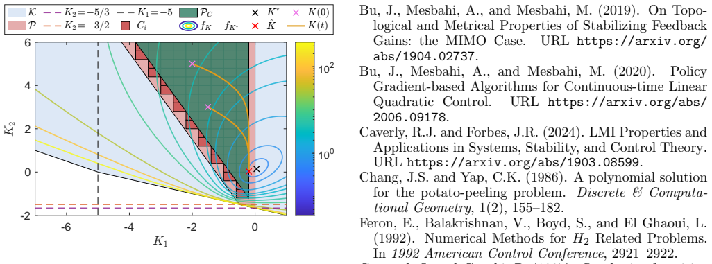
[Numerical examples] Numerical examples: the reported trajectories would be more informative if the polytope boundaries were overlaid on the gain space plots and if the achieved LQR cost were compared against the unconstrained LQR optimum (when feasible) or against a simple outer bound.
[Preliminaries] Notation: the distinction between strict passivity and passivity is used throughout but the precise matrix inequality (e.g., the strict version of the KYP lemma) is not restated in the main text; a short reminder equation would improve readability.

Simulated Author's Rebuttal

2 responses · 0 unresolved

We thank the referee for the constructive feedback and positive evaluation of the geometric properties and algorithmic approach. We address each major comment below, acknowledging the limitations identified and outlining the revisions we will make to clarify these points without overstating the method's guarantees.

read point-by-point responses

Referee: [Abstract / indirect approach] Abstract and the description of the indirect approach: the set of passivating gains is shown to be possibly nonconvex, so any compact convex polytope necessarily excludes feasible gains. No explicit construction of the polytope (e.g., via vertex enumeration or facet description) nor any quantitative guarantee (Hausdorff distance, volume ratio, or suboptimality bound on J(K_poly) - min J(K)) is supplied to ensure the retained point remains useful for the original constrained problem.

Authors: We agree that the possible nonconvexity of the passivating gain set means any convex inner approximation necessarily excludes some feasible gains. The manuscript describes the polytope as the convex hull of a finite collection of passivating gains chosen to satisfy the strict passivity LMI, but does not supply a general vertex-enumeration algorithm or facet description. Deriving a priori quantitative guarantees such as Hausdorff distance or suboptimality bounds is difficult in the absence of additional structural assumptions on the system, given the nonconvexity. In the revision we will expand the polytope-construction description with explicit details on vertex selection used in the examples, add a remark on the approximation's practical performance as observed numerically, and include a dedicated paragraph noting the lack of general bounds as a limitation of the indirect method. revision: partial
Referee: [Projected gradient flow] Description of the projected gradient flow: the LQR cost J(K) is a non-convex function of the gain (the Riccati/Lyapunov solution depends quadratically on K). Projected gradient flow over a convex set is guaranteed only to reach a stationary point; the manuscript provides no argument ruling out multiple distinct stationary values with materially different costs, nor any mechanism (e.g., multi-start, second-order test, or global-optimization subroutine) to identify the best point inside the polytope.

Authors: We concur that J(K) is non-convex in K because the Lyapunov solution depends quadratically on the gain, so projected gradient flow is guaranteed only to reach a stationary point that need not be globally optimal inside the polytope. The manuscript contains no analysis ruling out multiple stationary points with substantially different costs and no built-in mechanisms such as multi-start. In the revised manuscript we will add a paragraph discussing the non-convexity of the objective and the possibility of distinct stationary values. We will also recommend and illustrate the practical use of multiple random initializations inside the polytope (feasible because the set is convex and compact), followed by selection of the lowest-cost stationary point obtained. revision: yes

Circularity Check

0 steps flagged

No circularity; derivation self-contained on standard LTI/LQR primitives

full rationale

The paper derives properties of the passivating gain set directly from LTI dynamics and passivity definitions, then proposes an inner polytope approximation followed by projected gradient flow on the standard LQR cost. No equation or claim reduces to a self-definition, a fitted input relabeled as prediction, or a load-bearing self-citation chain. The central method rests on convex optimization primitives and the known nonconvexity of the feasible set, without any quantity being defined circularly in terms of its own output or a prior result by the same authors that itself lacks independent verification.

Axiom & Free-Parameter Ledger

0 free parameters · 1 axioms · 0 invented entities

The central claim rests on standard definitions of passivity and LQR for LTI systems together with basic properties of convex sets and gradient flows; no new free parameters, ad-hoc axioms, or invented entities are introduced in the abstract.

axioms (1)

domain assumption The closed-loop system is linear time-invariant and the passivity and LQR cost are defined via standard quadratic forms and storage functions.
Invoked when stating the objective and the bilinear matrix inequalities.

pith-pipeline@v0.9.0 · 5446 in / 1375 out tokens · 39897 ms · 2026-05-10T11:05:31.989280+00:00 · methodology

discussion (0)

Reference graph

Works this paper leans on

19 extracted references · 19 canonical work pages

[1]

and Vandenberghe, L

Balakrishnan, V. and Vandenberghe, L. (1995). Connec- tions Between Duality in Control Theory and Convex Optimization. InProceedings of 1995 American Control Conference, volume 6, 4030–4034

work page 1995
[2]

(2020).Dissipative Systems Analysis and Control

Brogliato, B., Lozano, R., Maschke, B., and Egeland, O. (2020).Dissipative Systems Analysis and Control

work page 2020
[3]

Bu, J., Mesbahi, A., and Mesbahi, M. (2019). On Topo- logical and Metrical Properties of Stabilizing Feedback Gains: the MIMO Case. URLhttps://arxiv.org/ abs/1904.02737

work page Pith review arXiv 2019
[4]

Bu, J., Mesbahi, A., and Mesbahi, M. (2020). Policy Gradient-based Algorithms for Continuous-time Linear Quadratic Control. URLhttps://arxiv.org/abs/ 2006.09178

work page arXiv 2020
[5]

and Forbes, J.R

Caverly, R.J. and Forbes, J.R. (2024). LMI Properties and Applications in Systems, Stability, and Control Theory. URLhttps://arxiv.org/abs/1903.08599

work page arXiv 2024
[6]

and Yap, C.K

Chang, J.S. and Yap, C.K. (1986). A polynomial solution for the potato-peeling problem.Discrete & Computa- tional Geometry, 1(2), 155–182

work page 1986
[7]

Feron, E., Balakrishnan, V., Boyd, S., and El Ghaoui, L. (1992). Numerical Methods forH 2 Related Problems. In1992 American Control Conference, 2921–2922

work page 1992
[8]

and Gapski, P

Geromel, J. and Gapski, P. (1997). Synthesis of positive realH 2 controllers.IEEE Transactions on Automatic Control, 42(7), 988–992

work page 1997
[9]

Haddad, W., Bernstein, D., and Wang, Y. (1994). Dissipa- tiveH 2 /H ∞ controller synthesis.IEEE Transactions on Automatic Control, 39(4), 827–831

work page 1994
[10]

Hallinan, L., Watson, J.D., and Lestas, I. (2025). Inverse Optimal Control for Passive Network Systems.IEEE Trans. Autom. Control, 70(10), 6969–6976

work page 2025
[11]

and Johnson, C.R

Horn, R.A. and Johnson, C.R. (2012).Matrix Analysis. Cambridge University Press, 2 edition

work page 2012
[12]

and Stein, O

Jongen, H.T. and Stein, O. (2003). Constrained global optimization: Adaptive gradient flows. InFrontiers in Global Optimization, volume 74, 223–236. Springer

work page 2003
[13]

(2002).Nonlinear Systems

Khalil, H.K. (2002).Nonlinear Systems. Prentice Hall, Upper Saddle River, N.J., 3 edition. L¨ ofberg, J. (2012). Automatic robust convex program- ming.Optim. Methods Softw., 27(1), 115–129

work page 2002
[14]

and Joshi, S

Lozano-Leal, R. and Joshi, S. (1988). On the design of the dissipative LQG-type controllers. InProc. IEEE Conf. Decis. Control, volume 2, 1645–1646

work page 1988
[15]

and Adamy, J

Madeira, D.d.S. and Adamy, J. (2016). On the Equivalence Between Strict Positive Realness and Strict Passivity of Linear Systems.IEEE Transactions on Automatic Control, 61(10), 3091–3095

work page 2016
[16]

Peaucelle, D., Fradkov, A., and Andrievsky, B. (2005). Ro- bust passification via static output feedback-lmi results. IF AC Proceedings Volumes, 38(1), 820–825

work page 2005
[17]

and Pullen, S.P

Shimomura, T. and Pullen, S.P. (2002). Strictly positive realH 2 controller synthesis via iterative algorithms for convex optimization.Journal of guidance, control, and dynamics, 25(6), 1003–1011

work page 2002
[18]

Su, L., Gupta, V., and Antsaklis, P. (2020). Feedback passivation of linear systems with fixed-structure con- trollers.IEEE Control Systems Letters, 4(2), 498–503

work page 2020
[19]

Sun, W., Khargonekar, P., and Shim, D. (1994). Solution to the positive real control problem for linear time- invariant systems.IEEE Trans. Autom. Control, 39(10), 2034–2046

work page 1994

[1] [1]

and Vandenberghe, L

Balakrishnan, V. and Vandenberghe, L. (1995). Connec- tions Between Duality in Control Theory and Convex Optimization. InProceedings of 1995 American Control Conference, volume 6, 4030–4034

work page 1995

[2] [2]

(2020).Dissipative Systems Analysis and Control

Brogliato, B., Lozano, R., Maschke, B., and Egeland, O. (2020).Dissipative Systems Analysis and Control

work page 2020

[3] [3]

Bu, J., Mesbahi, A., and Mesbahi, M. (2019). On Topo- logical and Metrical Properties of Stabilizing Feedback Gains: the MIMO Case. URLhttps://arxiv.org/ abs/1904.02737

work page Pith review arXiv 2019

[4] [4]

Bu, J., Mesbahi, A., and Mesbahi, M. (2020). Policy Gradient-based Algorithms for Continuous-time Linear Quadratic Control. URLhttps://arxiv.org/abs/ 2006.09178

work page arXiv 2020

[5] [5]

and Forbes, J.R

Caverly, R.J. and Forbes, J.R. (2024). LMI Properties and Applications in Systems, Stability, and Control Theory. URLhttps://arxiv.org/abs/1903.08599

work page arXiv 2024

[6] [6]

and Yap, C.K

Chang, J.S. and Yap, C.K. (1986). A polynomial solution for the potato-peeling problem.Discrete & Computa- tional Geometry, 1(2), 155–182

work page 1986

[7] [7]

Feron, E., Balakrishnan, V., Boyd, S., and El Ghaoui, L. (1992). Numerical Methods forH 2 Related Problems. In1992 American Control Conference, 2921–2922

work page 1992

[8] [8]

and Gapski, P

Geromel, J. and Gapski, P. (1997). Synthesis of positive realH 2 controllers.IEEE Transactions on Automatic Control, 42(7), 988–992

work page 1997

[9] [9]

Haddad, W., Bernstein, D., and Wang, Y. (1994). Dissipa- tiveH 2 /H ∞ controller synthesis.IEEE Transactions on Automatic Control, 39(4), 827–831

work page 1994

[10] [10]

Hallinan, L., Watson, J.D., and Lestas, I. (2025). Inverse Optimal Control for Passive Network Systems.IEEE Trans. Autom. Control, 70(10), 6969–6976

work page 2025

[11] [11]

and Johnson, C.R

Horn, R.A. and Johnson, C.R. (2012).Matrix Analysis. Cambridge University Press, 2 edition

work page 2012

[12] [12]

and Stein, O

Jongen, H.T. and Stein, O. (2003). Constrained global optimization: Adaptive gradient flows. InFrontiers in Global Optimization, volume 74, 223–236. Springer

work page 2003

[13] [13]

(2002).Nonlinear Systems

Khalil, H.K. (2002).Nonlinear Systems. Prentice Hall, Upper Saddle River, N.J., 3 edition. L¨ ofberg, J. (2012). Automatic robust convex program- ming.Optim. Methods Softw., 27(1), 115–129

work page 2002

[14] [14]

and Joshi, S

Lozano-Leal, R. and Joshi, S. (1988). On the design of the dissipative LQG-type controllers. InProc. IEEE Conf. Decis. Control, volume 2, 1645–1646

work page 1988

[15] [15]

and Adamy, J

Madeira, D.d.S. and Adamy, J. (2016). On the Equivalence Between Strict Positive Realness and Strict Passivity of Linear Systems.IEEE Transactions on Automatic Control, 61(10), 3091–3095

work page 2016

[16] [16]

Peaucelle, D., Fradkov, A., and Andrievsky, B. (2005). Ro- bust passification via static output feedback-lmi results. IF AC Proceedings Volumes, 38(1), 820–825

work page 2005

[17] [17]

and Pullen, S.P

Shimomura, T. and Pullen, S.P. (2002). Strictly positive realH 2 controller synthesis via iterative algorithms for convex optimization.Journal of guidance, control, and dynamics, 25(6), 1003–1011

work page 2002

[18] [18]

Su, L., Gupta, V., and Antsaklis, P. (2020). Feedback passivation of linear systems with fixed-structure con- trollers.IEEE Control Systems Letters, 4(2), 498–503

work page 2020

[19] [19]

Sun, W., Khargonekar, P., and Shim, D. (1994). Solution to the positive real control problem for linear time- invariant systems.IEEE Trans. Autom. Control, 39(10), 2034–2046

work page 1994