pith. machine review for the scientific record. sign in

arxiv: 2604.25463 · v1 · submitted 2026-04-28 · ✦ hep-th · math-ph· math.MP· math.RT

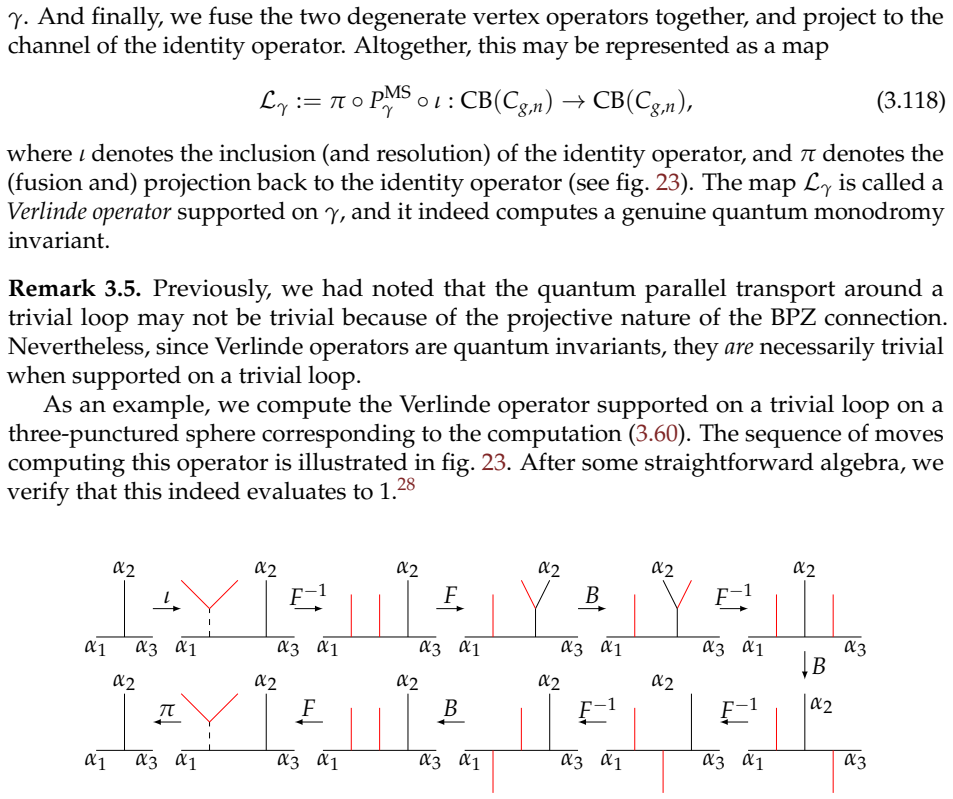
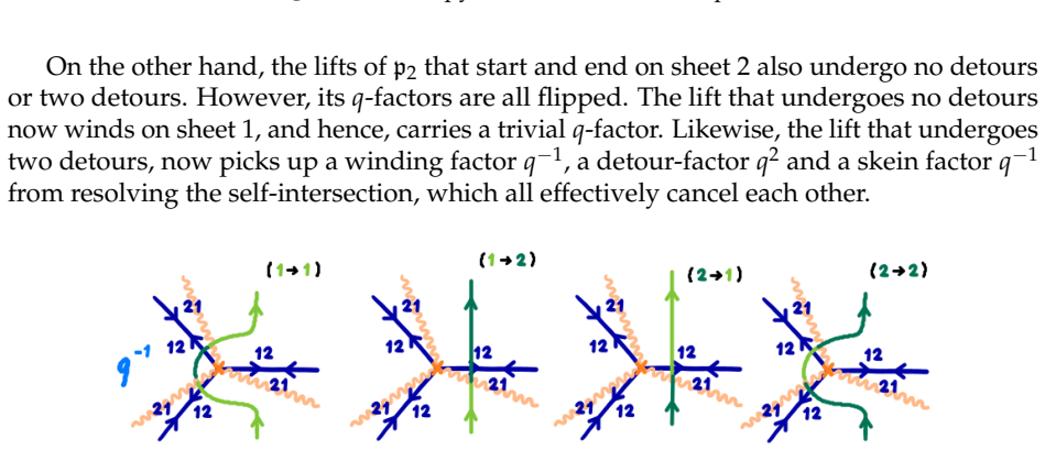
Recognition: unknown

Liouville Blocks from Spectral Networks

Authors on Pith no claims yet

Pith reviewed 2026-05-07 15:55 UTC · model grok-4.3

classification ✦ hep-th math-phmath.MPmath.RT
keywords Liouville theoryspectral networksconformal blocksFenchel-Nielsen networksMaulik-Okounkov R-matrixwall-crossingGoncharov-Shen blocksq-nonabelianisation
0
0 comments X

The pith

Spectral networks extended by the Maulik-Okounkov R-matrix generate the full spectrum of Liouville conformal blocks.

A machine-rendered reading of the paper's core claim, the machinery that carries it, and where it could break.

The paper develops a formalism based on spectral networks of Fenchel-Nielsen type to study quantum Liouville theory. It first constructs q-parallel transport via q-nonabelianisation and checks consistency with the Moore-Seiberg formalism. The standard free-field approach with integration contours is shown to miss wall-crossing effects. Extending the free-field method to smooth spectral coverings, with the Maulik-Okounkov R-matrix handling the quantum corrections, leads to the conjecture that every Liouville block is produced and that Goncharov-Shen blocks receive a first-principles definition.

Core claim

By extending the free-field formalism to smooth spectral coverings and employing the Maulik-Okounkov R-matrix, the construction generates the entire spectrum of Liouville conformal blocks and supplies a first-principle definition for Goncharov-Shen conformal blocks.

What carries the argument

Fenchel-Nielsen spectral networks combined with q-nonabelianisation and the Maulik-Okounkov R-matrix acting on smooth spectral coverings to capture wall-crossing.

If this is right

  • The full spectrum of Liouville conformal blocks is generated systematically from the spectral network construction.
  • Goncharov-Shen conformal blocks acquire a definition directly from the extended free-field method.
  • All wall-crossing phenomena are accounted for by the action of the Maulik-Okounkov R-matrix.
  • Quantum parallel transport on these networks matches the Moore-Seiberg results.

Where Pith is reading between the lines

These are editorial extensions of the paper, not claims the author makes directly.

  • The same construction may supply a uniform method for generating blocks in related theories such as Toda CFT.
  • Direct links between spectral networks and the integrable structure of Liouville theory become available for explicit computation.
  • Testing the formalism on higher-genus surfaces with known block expressions would provide a concrete check.

Load-bearing premise

That extending the free-field formalism to smooth spectral coverings with the Maulik-Okounkov R-matrix fully captures all wall-crossing effects and produces every Liouville block without missing sectors.

What would settle it

Compute a Liouville block for a specific Fenchel-Nielsen network that crosses walls using the extended formalism and compare the result to an independent Moore-Seiberg calculation; any mismatch falsifies the conjecture.

Figures

Figures reproduced from arXiv: 2604.25463 by Lotte Hollands, Subrabalan Murugesan.

Figure 1
Figure 1. Figure 1: Left: FG network on the 3-punctured sphere, with punctures at z = ±1 and z = ∞, for ϕ2 = (z 2+1) (z 2−1) 2 (dz) 2 at ϑ = π 2 . Labelings are fixed with respect to the choice of trivialisation λ1 = √ −z 2 − 1/(z 2 − 1) and λ2 = − √ −z 2 − 1/(z 2 − 1). Right: same network together with the dual ideal triangulation (in dashed light blue). On the other hand, for certain phases, all ij−trajectories (critical an… view at source ↗
Figure 2
Figure 2. Figure 2: Left: Picture of a Fenchel-Nielsen type spectral network on the 3-punctured sphere, with punctures at z = ±1 and z = ∞, for ϕ2 = (z 2+1) (z 2−1) 2 (dz) 2 at ϑ = 0. Right: same spectral network together with the dual pair of pants decomposition (in dashed red). Fenchel-Nielsen molecules FN networks on the 3-punctured sphere P1 0,1,∞ can be gener￾ated by the quadratic differential ϕ2 = − µ 2 ∞z 2 − (µ 2 ∞ + … view at source ↗
Figure 3
Figure 3. Figure 3: Picture of a Fenchel-Nielsen type spectral network (in dark blue) on the 4- punctured sphere, with punctures at z = 0, 0.2, 1 and ∞, for ϕ2 = 2.6−2.94z+15.04z 2−14.7z 3+6.5z 4 z 2(z−0.2) 2(z−1) 2 at ϑFN = 0. The dual pants decomposition (in dashed red) separates the punctures at z = 0 and 0.2 from those at z = 1 and ∞. Note that we can align the orientation of saddle trajecto￾ries in both molecules by addi… view at source ↗
Figure 4
Figure 4. Figure 4: Fenchel-Nielsen type networks on the 3-punctured sphere with quadratic differen￾tial from eq. (2.6) with µk > 0. Left: molecule I with µ0 + µ1 > µ∞. Right: molecule II with µ0 + µ1 < µ∞. There are two versions of each molecule, related by exchanging the labels 1 ↔ 2 view at source ↗
Figure 5
Figure 5. Figure 5: A degenerate spectral network of Fenchel-Nielsen type on the three-punctured sphere, with punctures at z = ±1 and z = ∞, for ϕ2 = z 2 (z 2−1) 2 (dz) 2 at ϑ = 0. Higher rank spectral networks In this paper we mostly focus on spectral networks of rank 2. Yet, we believe most of the discussions can be extended to higher rank spectral networks, and they do come up explicitly in §5.4. We therefore introduce the… view at source ↗
Figure 6
Figure 6. Figure 6: Cartoon of spectral network on the 4-punctured sphere for the same quadratic differential ϕ2 as in fig. 3, but now with ϑ = η > 0 deviating slightly from the Fenchel-Nielsen phase. The red loop is a choice of pants cycle. The cartoon highlights all trajectories (in bright blue) that start in the left pair of pants and de-emphasises all trajectories (in light blue) that start in the right pair of pants. The… view at source ↗
Figure 7
Figure 7. Figure 7: Example of a flip transition of an FG-type spectral network. for γ ′ ̸= γ. The spectral coordinates {X FN γ } associated to a spectral network of FN-type can be identified with (the exponential of) complexified Fenchel-Nielsen length-twist coordinates [25]. Indeed, the SL(2, C)-monodromy around a pants cycle a is diagonal in terms of the spectral coordinates X FN A , where A is a lift of a, since the W-abe… view at source ↗
Figure 8
Figure 8. Figure 8: Example of a detour path (in light green), starting on sheet 1 and ending on sheet 2 of the covering Σ. Consider, for example, an open path p on C that crosses an ij-trajectory of the spectral network W. Then the collection of lifts of p to the cover contains the two canonical lifts of p to each sheet of the covering, i.e. the direct lifts, as well as precisely one detour path that runs from sheet i to she… view at source ↗
Figure 9
Figure 9. Figure 9: When gauging a puncture we cut out a small open disc around the puncture and fix the trivialisation of the bundle E at a marked point on the boundary of the open disc. As a result, the abelian holonomies along the paths Ak and Bk on Σ turn into new spectral coordinates. along one boundary component (of a gauged 3-sphere) is the same as along another bound￾ary component (of possibly a different gauged 3-sph… view at source ↗
Figure 10
Figure 10. Figure 10: Choice of a trivialisation of Σ (in light orange) and a path groupoid (in light grey) with respect to the Fenchel-Nielsen type molecule I. We gauge each puncture by fixing a trivialisation at the marked points labeled by A, B and C (in red). The S-matrices (in light blue), attributed to each crossing with a double trajectory (in dark blue) are labeled by S1, S2 and S3. and 2, and anti-clockwise for punctu… view at source ↗
Figure 11
Figure 11. Figure 11: From left to right: spectral network W− FN (in dark blue) at increasing values of the (real) mass filtration parameter µ = e −iϑ R w √ ϕ2 [18]. Lightest detour path (in light green) on the left, and next-to-lightest detour path (in light green) on the right. The two infinite families of detour paths described in the text appear when increasing µ further. We find the relation between the spectral coordinat… view at source ↗
Figure 12
Figure 12. Figure 12: Choice of path groupoid (in light grey and red) on 4-punctured sphere. The little black arrows indicate the orientations of 1-cycles around punctures and pants curve. XA and XB are the abelian parallel transports along the A-cycle (in red) and the B-cycle (in purple) on Σ, respectively. T ij kl is the abelian parallel transport along an open path p ij kl ⊂ Σ which runs from the lift of the marked point fo… view at source ↗
Figure 13
Figure 13. Figure 13: The three standard choices of bases for a four-point conformal block. different pair of pants decompositions of Cg,n and the edges/morphisms are actions of the generators. This groupoid is known as the Moore-Seiberg groupoid. Starting with a given pair of pants decomposition P, there may be several different sequences of basic moves leading to another decomposition P ′ . Such consistency relations between… view at source ↗
Figure 14
Figure 14. Figure 14: The action of the Moore-Seiberg moves on Liouville blocks. Figures (a) and (b) illustrate the fusion and inverse fusion moves, respectively. Figure (c) illustrates the braiding move. where the coefficient B α3α2 α = exp(−iπ(∆(α) − ∆(α2) − ∆(α3))) (3.50) is merely a complex number. The twisting action should be thought of as transporting α3 around α2 in the clockwise direction. The fusion matrices are gene… view at source ↗
Figure 15
Figure 15. Figure 15: A 4-point conformal block with one degenerate operator (in red) inserted is shown in both s- and t-channel. Here, α = α1 ± b/2 and α ′ = α2 ± b/2. we have that [59] 18 F++  α2 −b/2 α3 α1  = Γ[b(2α1 − b)]Γ[b(Q − 2α2)] Γ[b(α1 − α2 + α3 − b 2 )]Γ[b(α1 − α2 − α3 + Q − b 2 )] , (3.52) and, F−+  α2 −b/2 α3 α1  = F++  α2 −b/2 α3 Q − α1  , F+−  α2 −b/2 α3 α1  = F++  Q − α2 −b/2 α3 α1  , and F−−  α2 −b/… view at source ↗
Figure 16
Figure 16. Figure 16: The fusion and braiding matrices correspond to parallel transport of the q￾hypergeometric equation on the 3-punctured sphere. You may recognise the fusion matrices Fss′ in equation (3.55) as the connection matrices for the hypergeometric differential equation. The braiding matrices Bss′ in eq. (3.59) agree with this interpretation up to the factor of q 1/2. Indeed, the Lax equation on the 3-punctured sphe… view at source ↗
Figure 17
Figure 17. Figure 17: Conformal block computation corresponding to moving the degenerate vertex operator V1,2(z) along a trivial loop on the 3-punctured sphere. Indeed, suppose we consider the BPZ equation (or null-vector decoupling equation) for the four-point conformal block F Vir 1,2 (z)  z(1 − z) b 2 ∂ 2 z + (2z − 1)∂z + ∆1,2 + ∆1 z − ∆4 + ∆2 1 − z  F Vir 1,2 (z) = 0 (3.61) as a standard Fuchsian ODE on the 3-punctured s… view at source ↗
Figure 18
Figure 18. Figure 18: The 1-cycles Ab and Bb on the covering Σ of the 3-punctured sphere. Remark 3.4. We should be mindful about the following. The Lax connection ∇Lax on the gauged 3-sphere reduces to Riemann’s connection ∇Rie on the 3-punctured sphere, but is not strictly equal to it. In the limit where we ”ungauge” the punctures, the superpotential on the gauged 3-sphere simplifies to the superpotential on the 3-punctured s… view at source ↗
Figure 19
Figure 19. Figure 19: A five-point conformal block including a single degenerate insertion on the 4-punctured sphere with a marked point. The internal momenta α and α ′ differ by ±b/2. The internal momentum through the pants cycle depends on which side of the pants tube the degenerate operator is inserted. If it is inserted to the left the internal momentum through the pants cycle is α, whereas if it is moved to the right of t… view at source ↗
Figure 20
Figure 20. Figure 20: Path β on the 4-punctured sphere, with base-point just above the marked point labeled a. 3.3.1 Example: 4-punctured sphere Let us, for instance, compute the Moore-Seiberg monodromy along the path β = pa2 ◦ a2 ◦ p −1 a2 ◦ pa3 ◦ a −1 3 ◦ p −1 a3 (3.100) on the 4-punctured sphere, as illustrated in fig. 20. Semi-classically, this monodromy is computed from Heun’s equation, which takes up the role of the Lax … view at source ↗
Figure 21
Figure 21. Figure 21: Computation of the quantum parallel transport P MS β of a degenerate operator (in red) around the 1-cycle β on the four-punctured sphere, illustrated in fig. 20. The quantum result can instead be computed through the sequence of moves shown in fig. 21. Assuming that the degenerate operator is initially inserted to the left of the pants tube, with internal momentum α, the quantum parallel transport along t… view at source ↗
Figure 22
Figure 22. Figure 22: Two punctures (possibly within the same surface) can be glued together if they carry conjugate momenta α and Q − α, respectively. This is because after reversing the orientation of one of the momenta, this momentum is flowing in the same direction with the same magnitude as the other momentum. Aside: parallel transport versus monodromy invariants Our emphasis in this paper is on the quantum parallel trans… view at source ↗
Figure 23
Figure 23. Figure 23: Comb diagrams for the computation of the action of a Verlinde operator supported on a trivial loop inside a three-punctured sphere. The dashed lines represent the identity operator and red lines represent the degenerate operators. 3.3.2 Quantum Fenchel-Nielsen coordinates Our aim in this section is to find out how the relation (3.85) between MS parallel trans￾port and parallel transport expressed in FN-ty… view at source ↗
Figure 24
Figure 24. Figure 24: On the left: the symmetry defect D (in dark blue) acts on the (extended) opera￾tor O (in red) by wrapping the support of the operator. On the right: the symmetry defect D′ acts on the (extended) operator O by moving through it. 3.4.2 Fenchel-Nielsen networks as symmetry defects We now argue that Fenchel-Nielsen type networks act as 0-form symmetry defects in Liouville theory, associated with its underlyin… view at source ↗
Figure 25
Figure 25. Figure 25: Leaf space (in yellow) for a simple FG spectral network (in blue) on the three￾punctured sphere. By making small perturbations if necessary, we assume that the projection of L onto the 3d leaf space WL 3d only has finitely many points of self-intersection and that L is generically 31At the Fenchel-Nielsen phase, the skein algebra is mapped into a localised quantum torus algebra in order to handle the infi… view at source ↗
Figure 26
Figure 26. Figure 26: On the left: an exchange occurs when a link L (in red) self-intersects upon projection to the 3d leaf space WL 3d (in yellow). In the middle: this is equivalent to two different segments of L crossing the same ij-trajectory (in light blue). On the right: in such case, depending on the orientations, the lifts L˜ (in light and dark green) of the two segments may exchange their strands. Both detour paths and… view at source ↗
Figure 27
Figure 27. Figure 27: If an upward-travelling detour L˜ (in light green) undergoes a clockwise (on the left), or anti-clockwise (on the right), detour along a critical ij−trajectory (in dark blue), it is accompanied by a factor of q −1/2 or q 1/2, respectively. For a downward-travelling detour, the q-factors are reversed view at source ↗
Figure 28
Figure 28. Figure 28: Locally, in a neighbourhood of a point of tangency, parametrise the base C by (real) coordinates x, y, in such a way that the WKB foliation is parallel to ∂y, and parametrise the height-direction by t. Then the projection of the link L to C, at this point of tangency, must be tangential to an ij-trajectory. • Each point of tangency of the link L receives an overall winding factor of q ±1/2 , depending on … view at source ↗
Figure 29
Figure 29. Figure 29: Any point of tangency of a link L (in red) contributes an overall winding factor, which depends both on the orientation of the link with respect to the ij−trajectory (in light blue) and on the tangency (up or down) of L. The illustrated q-factors are assigned to upward traveling links, they are reversed for downward traveling links view at source ↗
Figure 30
Figure 30. Figure 30: A point of tangency of the projection of a lift L˜ (in light green) contributes a sheet-dependent q-factor, which depends only on the orientation of the winding with respect to the ij-trajectory and the tangency (up or down) of L˜. The illustrated factors are assigned to upward travelling links, they are reversed for downward travelling links. lifts L˜. This means that we can repackage the overall and the… view at source ↗
Figure 31
Figure 31. Figure 31: Locally, detours either turn clockwise or anti-clockwise in the vicinity of the branch-point. In this figure we illustrate that a detour is always followed by a point of tangency. Using the rules of q-nonabelianisation, we verify that the two contributions to the total framing factor precisely cancel each other view at source ↗
Figure 32
Figure 32. Figure 32: The overall and the sheet-dependent winding factor can be combined into a single sheet-dependent q-factor. The illustrated factors are associated with upward travelling links; they are reversed for a downward travelling links. This implies that q-nonabelianisation essentially quantises trace functions on the moduli space of flat connections. However, in this paper we are more interested in quantum paralle… view at source ↗
Figure 33
Figure 33. Figure 33: Fully symmetric FN network (in dark blue) on the gauged 3-sphere, together with the base-points (in light blue) placed infinitesimally away on either side of the double walls. Consider the fully-symmetric FN molecule from fig. 10 on the gauged 3-sphere, which we have redrawn for convenience in fig. 33. The quantum FN S-matrix S qFN 2 is, by definition, 80 view at source ↗
Figure 34
Figure 34. Figure 34: We depict open paths corresponding to the generators Y 11 L , Y 12 L and Y ′12 L (drawn as projections to C × I). The paths start on the left base-point at t = 0 and run to the right base-point at t = 1. of S qFN. The other quantum FN S-matrices are similarly obtained by a cyclic permutation of the exponentiated masses and the corresponding open path generators. In principle, knowledge of the quantum S-ma… view at source ↗
Figure 35
Figure 35. Figure 35: Isotopy move across a double wall. The second path crosses the double wall twice. We may decompose this path into three parts labelled by ι, m and f , where ι labels the first part of the path that hasn’t crossed the wall yet, m labels the middle part in between the two crossings, and f labels the final 38The composition of a detour around different branch-points leads to a closed cycle around the two bra… view at source ↗
Figure 36
Figure 36. Figure 36: Equivalence between Y 11 ι Y 12 2,LY 22 m Y 21 2,RY 11 f (on the left) and Y 11 ι Y 11 2,LY 11 m Y 11 2,RY 11 f to￾gether with a closed loop around a branch-point (on the right). (We only show a single branch-cut to avoid clutter.) view at source ↗
Figure 37
Figure 37. Figure 37: Equivalence between Y 11 ι Y 11 2,LY 11 m Y 12 2,RY 22 f (on the left) and Y 11 ι Y 12 2,LY 22 m Y 22 2,RY 22 f (on the right) inside A. (We only show a single branch-cut to avoid clutter.) the q-nonabelianisation of the two paths p1 and p2, we simply count the q-factors of each lift. The (projections of the) various lifts of p1 are illustrated in fig. 39. The detours of the path p1 are captured by S qFN,… view at source ↗
Figure 38
Figure 38. Figure 38: Isotopy move across a branch-point. On the other hand, the lifts of p2 that start and end on sheet 2 also undergo no detours or two detours. However, its q-factors are all flipped. The lift that undergoes no detours now winds on sheet 1, and hence, carries a trivial q-factor. Likewise, the lift that undergoes two detours, now picks up a winding factor q −1 , a detour-factor q 2 and a skein factor q −1 fro… view at source ↗
Figure 39
Figure 39. Figure 39: Projections of the lifts of the open path p1 to C with source and target sheets indicated. Only the lift from sheet 1 to sheet 1 has a non-trivial q factor view at source ↗
Figure 40
Figure 40. Figure 40: Projections of the lifts of the open path p2 to C with source and target sheets indicated. The lifts of p2 that start on sheet 1 and end on sheet 2 either undergo a 1 → 2 detour at the “first wall” or a 2 → 1 detour at the “second wall” (see fig. 40). First of all, there is no q-contribution from self-intersections in this case. Second, the former lift has no detour-factor and winding factor while the lat… view at source ↗
Figure 41
Figure 41. Figure 41: On the left: example of a small loop (in green) around a simple branch-point, projected onto C. On the right: the same configuration (without the spectral network trajectories and the branch-cuts), but now projected onto a plane in C × I, perpendicular to one of the spectral network trajectories. 4.2.3 First-principle derivation We would now like to derive eq. (4.26) starting from the rules of q-nonabelia… view at source ↗
Figure 42
Figure 42. Figure 42: Decomposition of the lift ℓ1 (on the left) in terms of γ 1 and δℓ (on the right). (The path ℓ1 is a detour path in the British resolution of the FN molecule drawn in the background in light blue.) view at source ↗
Figure 43
Figure 43. Figure 43: Two different ways to decompose the open path on the left in terms of the quantum torus generators Xγ 1 , Xγ′ 1 and Y 11 zB . In §3.3.2, we learned that quantum spectral coordinates Xγ act as operators on the space of Liouville conformal blocks. In particular, the quantum generators Xγodd k , associated with odd 1-cycles γ odd k around the punctures zk , act by multiplication by the mass eigenvalues Mk . … view at source ↗
Figure 44
Figure 44. Figure 44: We can further write δℓ in terms of a detour δu around the upper branch-point. The first two figures show the 2d projections, and the last figure the 3d arrangement. We have suppressed two out of the three branch-cuts in the third figure for clarity. It is more convenient to write the detour around the bottom branch-point δℓ in terms of a detour around the top branch-point δu, as shown in fig. 44. This al… view at source ↗
Figure 45
Figure 45. Figure 45: Two representations γ (1) b and γ (2) b of the 1-cycle γb in the presence of the open path δu. The rest of the exercise is similar in nature: we find a decomposition of every possible lift in our preferred basis for the space of open skeins A on Σ, and evaluate the closed generators to get masses Mk . This is a straightforward exercise in abelian skein theory. We find that P q,+ ε ⇝   Y 11,+ ε 1−M−1 1 … view at source ↗
Figure 46
Figure 46. Figure 46: Since the path pb extends between two marked points on C, the abelian parallel transports along all the lifts of pb are gauge-invariant. 4.3.1 Physical interpretation: action on conformal blocks In §4.1.3, we realised the quantum torus generators Xγ as abelian Verlinde operators (i.e. Heisenberg-Verlinde operators) on the space of abelian conformal blocks on Σ. 41 Similarly, the 3d Chern-Simons picture al… view at source ↗
Figure 47
Figure 47. Figure 47: Geometric representation of the cup and cap maps ι ab and π ab that describe the fusion product between an abelian degenerate vertex operator and its conjugate. Upon quantisation, the fibre at zb is realised in terms of the identity open path Y ii zb and the dual fibre at z ′ b in terms of the conjugate path (Y ii z ′ b ) ∗ , which is simply the open path Y ii z ′ b running in the opposite direction. The … view at source ↗
Figure 48
Figure 48. Figure 48: Geometric representation of the operators ι ab α and π ab α that describe the fusion product between a generic abelian vertex operator and an abelian degenerate vertex operator. Suppose that ebp interpolates between marked points near punctures pi and pf . The quantum torus generator X ij bp can then be computed by first applying the wedge operator ι ab αi at the starting point, then the open path generat… view at source ↗
Figure 49
Figure 49. Figure 49: The skein diagram corresponding to the quantum torus generator X ij ebp for an open path eb ij p running between punctures pi and pf . α α ′ α = α view at source ↗
Figure 50
Figure 50. Figure 50: For a based loop in Σ, the operation π ab α ◦ Y ◦ ι ab α is the same as the operation π ab ◦ Y ◦ ι ab . path on C. Since q-nonabelianisation is a local procedure, the q-parallel transport along p may be computed by decomposing the path p as p = pゎpず · · · pり, (4.90) where each pろ is an (connected) open path embedded in a single pair of pants. Since the knowledge of the quantum FN S-matrix is sufficient to… view at source ↗
Figure 51
Figure 51. Figure 51: Ordering of the lifts of the pants-cycle γ and an open 1-cycle around a gauged puncture on Σ view at source ↗
Figure 52
Figure 52. Figure 52: There is no canonical way to order the lifts of closed pants-cycles in the presence of an open path. The two possible choices differ by factor of q ±2 . Indeed, let us see what happens to the definition of the mass eigenvalues as we move a pants cycle across an open path. Suppose the open path originates on sheet 1 in Σ × {0}. Then the pants cycles γleft and γright (denoted γ and γ ′ previously) on either… view at source ↗
Figure 53
Figure 53. Figure 53: The path β on the 4-punctured sphere is split into two paths βL and βR, each of which is decomposed into three pieces ι, d and f . where ∆ ±1 q (M) = q ±1M (4.96) is a difference operator acting on the length coordinate M, and the superscript ”op” denotes orientation reversal across the pants tube. Note that ∆q is precisely the difference operator Tb that we encountered in eq. (3.114). That is, q-parallel… view at source ↗
Figure 54
Figure 54. Figure 54: The winding of the diagonal path d with respect to the FN foliation. Comparing this expression with (the evaluation of) eq. (4.100), we note that the MS parallel transport and q-parallel transport agree in form, up to the overall winding factor, if we redefine the open path generators by half-integral powers of q as Yb11 βR := q 1 2Y 11 βR , Yb22 βR := q −1 2Y 22 βR , Yb12 βR := q −1 2Y 12 βR , Yb21 βR :=… view at source ↗
Figure 55
Figure 55. Figure 55: Left: degenerate network Wϑ=0 deg . Right: resolved spectral network Wϑ=0 (µ). Changing the phase ϑ 7→ ϑ + π exchanges the labels 12 ↔ 21. The matrix model partition function is given by Z β−mat ϑ = 1 N! Z Γϑ N ∏s=1 dys ∏ 1≤s<t≤N (ys − yt) 2β N ∏s=1 exp  y 2 s h¯  , (5.76) where ϑ = arg(h¯). Note that this has the form of Mehta’s integral. Specifically, at ϑ = π, when ¯h = −h < 0, we may choose the inte… view at source ↗
Figure 56
Figure 56. Figure 56: Degenerate networks defined by ϕ sing 2 in eq. (5.99) for µ0 = µ1 = 1. Left: At phase ϑ = π/2 the network is of degenerate Fenchel-Nielsen type. Middle: For phases π/2 < ϑ < π the network starts to unwind itself. Right: The network is at the simplest at ϑ = π (mod π). as the integration cycle at phase ϑ = 0. The matrix model partition function (5.101) is then computed by Selberg’s integral formula (B.13).… view at source ↗
Figure 57
Figure 57. Figure 57: Degenerate network of Fenchel-Nielsen type defined by ϕ2 in eq. (5.127) for µ0 = µq = µ1 = 1 and q = 1/5 at phase ϑ = π/2. Note that the spectral network at ϑ = π/2 (mod π) is of FN-type with respect to the pants decomposition whose pants cycle is going around the punctures at y = 0 and y = q. This is because we have chosen all µk > 0. Other pants decompositions can be obtained by changing the signs of th… view at source ↗
Figure 58
Figure 58. Figure 58: Degenerate network of Fock-Goncharov type defined by ϕ2 in eq. (5.127) for µ0 = µq = µ1 = 1 and q = 1/5 at phase ϑ = π. The two extended 21-trajectories run along the intervals [0, q] and [q, 1], respectively. At phase ϑ = 0 the network is the same with swapped labels 12 ↔ 21. Fock-Goncharov phase The simplest FG type network is found at ϑ = 0 and illustrated in fig. 58. The associated matrix model partit… view at source ↗
Figure 59
Figure 59. Figure 59: Two flip transitions connecting FG networks defined by ϕ2 in eq. (5.127) for µ0 = µq = µ1 = 1 and q = 1/5 at phase ϑ = −0.75π, ϑ = −0.68π and ϑ = −0.57π, respectively. These are the first two of an infinite series of flip transitions resulting in the FN-type network at phase ϑ = 0. Flips The degenerate network Wϑ deg undergoes an infinite series of flips when varying the phase ϑ from −π to −π/2. The first… view at source ↗
Figure 60
Figure 60. Figure 60: The Maulik-Okounkov R-matrix R1,2 intertwines the free-field realisation Vir(1) (with background charge +Q) on sheet 1 with the free-field realisation Vir(2) (with back￾ground charge −Q) on sheet 2 of the double covering Σ → C. Fortunately, it is well-known that there exists a free-field operator which does just that. It is called the Maulik-Okounkov (MO) R-matrix [44] 58 and defined through the relations… view at source ↗
Figure 61
Figure 61. Figure 61: The abelianisation of the vertex operator Vα(z) on the base C into the tensor product of Ve (1) α (z (1) ) and Ve (2) α (z (2) ) on the cover Σ. The arrows in this figure will be explained in the next paragraph. 143 view at source ↗
Figure 62
Figure 62. Figure 62: Relation between the singular and the MO abelianisation from the perspective of the cover Σ. On the left we start in the global free-field realisation, where (lifted) branch-cuts are dressed with the R-matrix R1,2. We write R1,2 = (12) RLiou and move the line defects labelled by RLiou towards each other. These line defects annihilate each other, while in the process conjugating all abelian vertex operator… view at source ↗
Figure 63
Figure 63. Figure 63: On the left: CFT abelianisation setup with respect to the MO orientation. On the right: CFT abelianisation setup with respect to the standard orientation. Comparison with the c = 1 abelianisation map In the following, we interpret the abelianisation map (5.168) as a deformation of the c = 1 abelianisation map proposed in [35]. Consider the free boson theory φe with background charge Q = 0 on Σ. In this ca… view at source ↗
Figure 64
Figure 64. Figure 64: CFT abelianisation of the screening charges Qij on the base C in terms of the screening charges Se (i) ± on the cover Σ. Suppose we conjugate the screening charges Seab ± on the second sheet (with respect to the background charge −Q on that sheet) to obtain the screening charges in the standard orientation. This leads to the expressions S ab + (z) = e bφe (z (1) ) ⊗ e −bφe (z (2) ) and S ab − (z) = e 1 b … view at source ↗
Figure 65
Figure 65. Figure 65: Through CFT abelianisation the nonabelian parallel transport associated with the degenerate vertex operator V1,2(z) crossing a critical ij-trajectory on C can be described on sheet i of the covering in terms of the OPE of the lift Ve (i) 1,2 (z) with the relevant screening charge Se (i) ± . If the OPE is regular, the operator Ve (i) 1,2 (z) can simply move through the lift of the trajectory. But when the … view at source ↗
Figure 66
Figure 66. Figure 66: Front view of the double cover of the 3-punctured sphere with respect to an FG-type network. The global free-field representation on the cover is defined by inserting the R-matrix R1,2 when crossing the branch-cuts, by inserting abelianised vertex operators Ve (i) k at the lifts of the three punctures, and by inserting the screening charges Qij along the lifts the ij-trajectories. (Note that the vertex op… view at source ↗
Figure 67
Figure 67. Figure 67: Cartoon of spectral network on the 4-punctured sphere for the same quadratic differential ϕ2 as in fig. 3, but now with ϑ = η > 0 deviating slightly from the Fenchel-Nielsen phase. Observe that four trajectories (in different shades of bright blue) cross the pants cycle a = [p], which is added in red. Each of these four trajectories starts from a different branch￾point, and each of them ends at a distinct… view at source ↗
Figure 68
Figure 68. Figure 68: A Pochhammer contour starts above the singularity at z = 1, winds clockwise around z = 0, then clockwise around z = 1, then counter-clockwise around z = 0, and finally counter-clockwise around z = 1. When R → ∞ the integrals along the large semi-circles tend to 0, and we find that Z C z α1−1 (1 − z) α2−1 dz =  e 2πi(α1+α2) − 1  Z c+i∞ c−i∞ z α1−1 (1 − z) α2−1 dz. (B.10) Substituting the Pochhammer integ… view at source ↗
read the original abstract

In this paper, we investigate the role of spectral networks in quantum Liouville theory, with particular emphasis on spectral networks of Fenchel-Nielsen-type. In the first part, we construct q-parallel transport for Fenchel-Nielsen networks through q-nonabelianisation, and compare with quantum parallel transport computed using the Moore-Seiberg formalism. This motivates a proposal for a quantum version of the NRS proposal. In the second part, we reproduce Liouville conformal blocks through the standard free-field formalism with Fenchel-Nielsen-type integration contours. However, we observe that this approach is not complete with respect to wall-crossing. We therefore develop an extension of the free-field formalism to smooth spectral coverings, with the Maulik-Okounkov R-matrix playing a central role. We conjecture that this new formalism generates the full spectrum of Liouville conformal blocks, and provides a first-principle definition for Goncharov-Shen conformal blocks.

Editorial analysis

A structured set of objections, weighed in public.

Desk editor's note, referee report, simulated authors' rebuttal, and a circularity audit. Tearing a paper down is the easy half of reading it; the pith above is the substance, this is the friction.

Referee Report

1 major / 1 minor

Summary. The manuscript investigates the role of spectral networks in quantum Liouville theory, with emphasis on Fenchel-Nielsen-type networks. In the first part, q-parallel transport is constructed for these networks through q-nonabelianisation and compared to quantum parallel transport from the Moore-Seiberg formalism, motivating a proposal for a quantum version of the NRS proposal. In the second part, Liouville conformal blocks are reproduced via the standard free-field formalism on Fenchel-Nielsen-type integration contours, but this approach is observed to be incomplete with respect to wall-crossing. An extension of the free-field formalism to smooth spectral coverings is developed, with the Maulik-Okounkov R-matrix playing a central role. The authors conjecture that this formalism generates the full spectrum of Liouville conformal blocks and provides a first-principle definition for Goncharov-Shen conformal blocks.

Significance. If the conjecture holds, the work would link spectral networks to the complete set of Liouville conformal blocks, potentially resolving wall-crossing incompleteness and supplying a first-principles definition for Goncharov-Shen blocks. The explicit construction of q-parallel transport via q-nonabelianisation and its direct comparison to the Moore-Seiberg formalism constitute a concrete strength, as does the clear identification of the incompleteness in the Fenchel-Nielsen free-field approach. These elements provide a solid basis for the proposed extension even while the completeness claim remains conjectural.

major comments (1)
  1. [Second part (extension to smooth spectral coverings)] In the second part, the free-field formalism on Fenchel-Nielsen contours is shown to be incomplete under wall-crossing, yet the extension to smooth spectral coverings via the Maulik-Okounkov R-matrix is conjectured to recover the full spectrum without any explicit matching computation or example demonstrating recovery of a previously missing block. This leaves the central completeness assumption unverified and load-bearing for the conjecture that the new formalism generates every Liouville block.
minor comments (1)
  1. [Abstract] The abstract would benefit from a sharper separation between the completed constructions (q-parallel transport comparison and FN reproduction) and the conjectural claims to improve readability.

Simulated Author's Rebuttal

1 responses · 0 unresolved

We thank the referee for their careful reading of our manuscript and for the positive evaluation of its strengths, including the explicit construction of q-parallel transport and the identification of incompleteness in the Fenchel-Nielsen approach. We address the major comment below.

read point-by-point responses
  1. Referee: [Second part (extension to smooth spectral coverings)] In the second part, the free-field formalism on Fenchel-Nielsen contours is shown to be incomplete under wall-crossing, yet the extension to smooth spectral coverings via the Maulik-Okounkov R-matrix is conjectured to recover the full spectrum without any explicit matching computation or example demonstrating recovery of a previously missing block. This leaves the central completeness assumption unverified and load-bearing for the conjecture that the new formalism generates every Liouville block.

    Authors: We agree that the completeness of the proposed extension is a conjecture without an explicit verification via a matching computation or example in the current manuscript. The extension is developed to address the observed incompleteness under wall-crossing by incorporating the Maulik-Okounkov R-matrix, which governs the transformations associated with the spectral network walls. This provides the structural reason for conjecturing that the full spectrum is recovered. We have added a clarifying paragraph in the revised manuscript to emphasize the conjectural nature of the completeness claim and to outline why the R-matrix is expected to generate the missing blocks. revision: partial

Circularity Check

0 steps flagged

No significant circularity; conjecture rests on external formalisms

full rationale

The paper constructs q-parallel transport via q-nonabelianisation and compares it to Moore-Seiberg, reproduces blocks with free-field methods on Fenchel-Nielsen contours while explicitly noting wall-crossing incompleteness, then extends the formalism using the external Maulik-Okounkov R-matrix to smooth coverings and states a conjecture that the extension yields the full spectrum plus a first-principles definition of Goncharov-Shen blocks. No equation or claim reduces by construction to a fitted input, self-definition, or load-bearing self-citation; all steps invoke independent external structures and the central claim is labeled as a conjecture rather than a closed derivation.

Axiom & Free-Parameter Ledger

0 free parameters · 1 axioms · 0 invented entities

Only the abstract is available, so the ledger is necessarily incomplete; the proposal relies on standard domain assumptions of quantum Liouville theory and spectral networks rather than new free parameters or invented entities.

axioms (1)
  • domain assumption The Maulik-Okounkov R-matrix correctly encodes the wall-crossing data needed to complete the free-field construction on smooth spectral coverings.
    This is the central new ingredient invoked to restore completeness with respect to wall-crossing.

pith-pipeline@v0.9.0 · 5466 in / 1480 out tokens · 66881 ms · 2026-05-07T15:55:41.425882+00:00 · methodology

discussion (0)

Sign in with ORCID, Apple, or X to comment. Anyone can read and Pith papers without signing in.

Reference graph

Works this paper leans on

109 extracted references · 4 canonical work pages

  1. [1]

    Two and three point functions in Liouville theory,

    H. Dorn and H. J. Otto, “Two and three point functions in Liouville theory,”Nucl. Phys. B, vol. 429, pp. 375–388, 1994

  2. [2]

    Structure constants and conformal bootstrap in Liouville field theory,

    A. B. Zamolodchikov and A. B. Zamolodchikov, “Structure constants and conformal bootstrap in Liouville field theory,”Nucl. Phys. B, vol. 477, pp. 577–605, 1996

  3. [3]

    On the Liouville three point function,

    J. Teschner, “On the Liouville three point function,”Phys. Lett. B, vol. 363, pp. 65–70, 1995

  4. [4]

    Liouville theory revisited,

    J. Teschner, “Liouville theory revisited,”Class. Quant. Grav., vol. 18, pp. R153–R222, 2001

  5. [5]

    On quantization of Liouville theory and related conformal field theories,

    J. A. Teschner, “On quantization of Liouville theory and related conformal field theories,” other thesis, 6 1995

  6. [6]

    Quantum Teichmuller space,

    L. Chekhov and V . V . Fock, “Quantum Teichmuller space,”Theor. Math. Phys., vol. 120, pp. 1245–1259, 1999

  7. [7]

    Integrability of liouville theory: proof of the dozz formula,

    A. Kupiainen, R. Rhodes, and V . Vargas, “Integrability of liouville theory: proof of the dozz formula,” 2019

  8. [8]

    Correlation functions in conformal Toda field theory. I.,

    V . A. Fateev and A. V . Litvinov, “Correlation functions in conformal Toda field theory. I.,”JHEP, vol. 11, p. 002, 2007. 176

  9. [9]

    Moduli spaces of local systems and higher teichm¨uller theory,

    V . Fock and A. Goncharov, “Moduli spaces of local systems and higher teichm¨uller theory,”Publications Math´ ematiques de l’IH´ES, vol. 103, pp. 1–211, 2006

  10. [10]

    Liouville Correlation Functions from Four-dimensional Gauge Theories,

    L. F. Alday, D. Gaiotto, and Y. Tachikawa, “Liouville Correlation Functions from Four-dimensional Gauge Theories,”Lett. Math. Phys., vol. 91, pp. 167–197, 2010

  11. [11]

    A(N-1) conformal Toda field theory correlation functions from confor- mal N = 2 SU(N) quiver gauge theories,

    N. Wyllard, “A(N-1) conformal Toda field theory correlation functions from confor- mal N = 2 SU(N) quiver gauge theories,”JHEP, vol. 11, p. 002, 2009

  12. [12]

    A slow review of the AGT correspondence,

    B. Le Floch, “A slow review of the AGT correspondence,”J. Phys. A, vol. 55, no. 35, p. 353002, 2022

  13. [13]

    The Ω deformed B-model for rigidN=2 theories,

    M.-x. Huang, A.-K. Kashani-Poor, and A. Klemm, “The Ω deformed B-model for rigidN=2 theories,”Annales Henri Poincare, vol. 14, pp. 425–497, 2013

  14. [14]

    A n-Triality,

    M. Aganagic, N. Haouzi, and S. Shakirov, “A n-Triality,” 3 2014

  15. [15]

    2D CFT blocks for the 4D classSk theories,

    V . Mitev and E. Pomoni, “2D CFT blocks for the 4D classSk theories,”JHEP, vol. 08, p. 009, 2017

  16. [16]

    Toda conformal blocks, quantum groups, and flat connections,

    I. Coman, E. Pomoni, and J. Teschner, “Toda conformal blocks, quantum groups, and flat connections,”Commun. Math. Phys., vol. 375, no. 2, pp. 1117–1158, 2019

  17. [17]

    Partition functions of non- Lagrangian theories from the holomorphic anomaly,

    F. Fucito, A. Grassi, J. F. Morales, and R. Savelli, “Partition functions of non- Lagrangian theories from the holomorphic anomaly,”JHEP, vol. 07, p. 195, 2023

  18. [18]

    Wall-crossing, Hitchin systems, and the WKB approximation,

    D. Gaiotto, G. W. Moore, and A. Neitzke, “Wall-crossing, Hitchin systems, and the WKB approximation,”Adv. Math., vol. 234, pp. 239–403, 2013

  19. [19]

    Spectral networks,

    D. Gaiotto, G. W. Moore, and A. Neitzke, “Spectral networks,”Annales Henri Poincare, vol. 14, pp. 1643–1731, 2013

  20. [20]

    Framed BPS States,

    D. Gaiotto, G. W. Moore, and A. Neitzke, “Framed BPS States,”Adv. Theor. Math. Phys., vol. 17, no. 2, pp. 241–397, 2013

  21. [21]

    Wall-Crossing in Coupled 2d-4d Systems,

    D. Gaiotto, G. W. Moore, and A. Neitzke, “Wall-Crossing in Coupled 2d-4d Systems,” JHEP, vol. 12, p. 082, 2012

  22. [22]

    BPS states in the Minahan-Nemeschansky E6 theory,

    L. Hollands and A. Neitzke, “BPS states in the Minahan-Nemeschansky E6 theory,” Commun. Math. Phys., vol. 353, no. 1, pp. 317–351, 2017

  23. [23]

    BPS states in the Minahan-Nemeschansky E7 theory,

    Q. Hao, L. Hollands, and A. Neitzke, “BPS states in the Minahan-Nemeschansky E7 theory,”JHEP, vol. 04, p. 039, 2020

  24. [24]

    Spectral Networks and Snakes,

    D. Gaiotto, G. W. Moore, and A. Neitzke, “Spectral Networks and Snakes,”Annales Henri Poincare, vol. 15, pp. 61–141, 2014

  25. [25]

    Spectral Networks and Fenchel–Nielsen Coordinates,

    L. Hollands and A. Neitzke, “Spectral Networks and Fenchel–Nielsen Coordinates,” Lett. Math. Phys., vol. 106, no. 6, pp. 811–877, 2016. 177

  26. [26]

    Kineider, G

    C. Kineider, G. Kydonakis, E. Rogozinnikov, V . Tatitscheff, and A. Thomas,Spectral Networks: Bridging higher-rank Teichm¨ uller theory and BPS states. 11 2024

  27. [27]

    Exact WKB and abelianization for the T3 equation,

    L. Hollands and A. Neitzke, “Exact WKB and abelianization for the T3 equation,” Commun. Math. Phys., vol. 380, no. 1, pp. 131–186, 2020

  28. [28]

    Higher length-twist coordinates, generalized Heun’s opers, and twisted superpotentials,

    L. Hollands and O. Kidwai, “Higher length-twist coordinates, generalized Heun’s opers, and twisted superpotentials,”Adv. Theor. Math. Phys., vol. 22, pp. 1713–1822, 2018

  29. [29]

    A geometric recipe for twisted superpoten- tials,

    L. Hollands, P . R¨uter, and R. J. Szabo, “A geometric recipe for twisted superpoten- tials,”JHEP, vol. 12, p. 164, 2021

  30. [30]

    Quantization of Integrable Systems and Four Dimensional Gauge Theories,

    N. A. Nekrasov and S. L. Shatashvili, “Quantization of Integrable Systems and Four Dimensional Gauge Theories,” in16th International Congress on Mathematical Physics, pp. 265–289, 2010

  31. [31]

    Darboux coordinates, Yang-Yang func- tional, and gauge theory,

    N. Nekrasov, A. Rosly, and S. Shatashvili, “Darboux coordinates, Yang-Yang func- tional, and gauge theory,”Nucl. Phys. B Proc. Suppl., vol. 216, pp. 69–93, 2011

  32. [32]

    Four Point Correlation Functions and the Operator Algebra in the Two-Dimensional Conformal Invariant Theories with the Central Charge c<1,

    V . S. Dotsenko and V . A. Fateev, “Four Point Correlation Functions and the Operator Algebra in the Two-Dimensional Conformal Invariant Theories with the Central Charge c<1,”Nucl. Phys. B, vol. 251, pp. 691–734, 1985

  33. [33]

    Conformal Algebra and Multipoint Correlation Functions in Two-Dimensional Statistical Models,

    V . S. Dotsenko and V . A. Fateev, “Conformal Algebra and Multipoint Correlation Functions in Two-Dimensional Statistical Models,”Nucl. Phys. B, vol. 240, p. 312, 1984

  34. [34]

    Toda Theories, Matrix Models, Topological Strings, and N=2 Gauge Systems,

    R. Dijkgraaf and C. Vafa, “Toda Theories, Matrix Models, Topological Strings, and N=2 Gauge Systems,” 9 2009

  35. [35]

    A new construction ofc=1 Virasoro blocks,

    Q. Hao and A. Neitzke, “A new construction ofc=1 Virasoro blocks,” 7 2024

  36. [36]

    Mathematical Structures of Non- perturbative Topological String Theory: From GW to DT Invariants,

    M. Alim, A. Saha, J. Teschner, and I. Tulli, “Mathematical Structures of Non- perturbative Topological String Theory: From GW to DT Invariants,”Commun. Math. Phys., vol. 399, no. 2, pp. 1039–1101, 2023

  37. [37]

    Exact WKB methods in SU(2) N f = 1,

    A. Grassi, Q. Hao, and A. Neitzke, “Exact WKB methods in SU(2) N f = 1,”JHEP, vol. 01, p. 046, 2022

  38. [38]

    org/abs/1904.10491(2022)

    A. Goncharov and L. Shen, “Quantum geometry of moduli spaces of local systems and representation theory,”arXiv preprint arXiv:1904.10491, 2019

  39. [39]

    Classical and Quantum Conformal Field Theory,

    G. W. Moore and N. Seiberg, “Classical and Quantum Conformal Field Theory,” Commun. Math. Phys., vol. 123, p. 177, 1989

  40. [40]

    Gauge Theory Loop Operators and Liouville Theory,

    N. Drukker, J. Gomis, T. Okuda, and J. Teschner, “Gauge Theory Loop Operators and Liouville Theory,”JHEP, vol. 02, p. 057, 2010. 178

  41. [41]

    Loop and surface operators in N=2 gauge theory and Liouville modular geometry,

    L. F. Alday, D. Gaiotto, S. Gukov, Y. Tachikawa, and H. Verlinde, “Loop and surface operators in N=2 gauge theory and Liouville modular geometry,”JHEP, vol. 01, p. 113, 2010

  42. [42]

    Generalized Global Symmetries,

    D. Gaiotto, A. Kapustin, N. Seiberg, and B. Willett, “Generalized Global Symmetries,” JHEP, vol. 02, p. 172, 2015

  43. [43]

    q-nonabelianization for line defects,

    A. Neitzke and F. Yan, “q-nonabelianization for line defects,”JHEP, vol. 09, p. 153, 2020

  44. [44]

    Quantum groups and quantum cohomology,

    D. Maulik and A. Okounkov, “Quantum groups and quantum cohomology,”arXiv preprint arXiv:1211.1287, 2012

  45. [45]

    The algebraic modular functor conjecture in type An quantum Teichm ¨uller theory,

    G. Schrader and A. Shapiro, “The algebraic modular functor conjecture in type An quantum Teichm ¨uller theory,”arXiv preprint arXiv:2509.03820, 2025

  46. [46]

    Quantum geometry and quiver gauge theories,

    N. Nekrasov, V . Pestun, and S. Shatashvili, “Quantum geometry and quiver gauge theories,”Commun. Math. Phys., vol. 357, no. 2, pp. 519–567, 2018

  47. [47]

    3d quantum trace map,

    S. Panitch and S. Park, “3d quantum trace map,” 2024

  48. [48]

    An embedding of skein algebras of surfaces into localized quantum tori from dehn-thurston coordinates,

    R. Detcherry and R. Santharoubane, “An embedding of skein algebras of surfaces into localized quantum tori from dehn-thurston coordinates,”Geometry & Topology, vol. 29, p. 313–348, Jan. 2025

  49. [49]

    Conformal matrix models as an alternative to conventional multimatrix models,

    S. Kharchev, A. Marshakov, A. Mironov, A. Morozov, and S. Pakuliak, “Conformal matrix models as an alternative to conventional multimatrix models,”Nucl. Phys. B, vol. 404, pp. 717–750, 1993

  50. [50]

    Conformal field theory techniques in random matrix models,

    I. K. Kostov, “Conformal field theory techniques in random matrix models,” in3rd Itzykson Meeting on Integrable Models and Applications to Statistical Mechanics, 7 1999

  51. [51]

    swn-plotter,

    A. Neitzke, “swn-plotter,” Mathematica program available at https://gauss.math.yale.edu/~an592/

  52. [52]

    Jenkins-Strebel differentials with poles.,

    J. Liu, “Jenkins-Strebel differentials with poles.,”Comment. Math. Helv., vol. 83(3), pp. 211—-240

  53. [53]

    Towards a 4d/2d correspondence for Sicilian quivers,

    L. Hollands, C. A. Keller, and J. Song, “Towards a 4d/2d correspondence for Sicilian quivers,”JHEP, vol. 10, p. 100, 2011

  54. [54]

    Topics in Liouville theory,

    L. Alvarez-Gaume and C. Gomez, “Topics in Liouville theory,” inSpring School on String Theory and Quantum Gravity (to be followed by Workshop), 7 1991

  55. [55]

    Minimal lectures on two-dimensional conformal field theory,

    S. Ribault, “Minimal lectures on two-dimensional conformal field theory,”SciPost Phys. Lect. Notes, vol. 1, p. 1, 2018

  56. [56]

    A guide to two-dimensional conformal field theory,

    J. Teschner, “A guide to two-dimensional conformal field theory,” 8 2017. 179

  57. [57]

    Generalized Lax and Backlund equations for Liouville and superLiou- ville theory,

    E. D’Hoker, “Generalized Lax and Backlund equations for Liouville and superLiou- ville theory,”Phys. Lett. B, vol. 264, pp. 101–106, 1991

  58. [58]

    Supersymmetric gauge theories, quantization of Mflat, and conformal field theory,

    J. Teschner and G. S. Vartanov, “Supersymmetric gauge theories, quantization of Mflat, and conformal field theory,”Adv. Theor. Math. Phys., vol. 19, pp. 1–135, 2015

  59. [59]

    Infinite Conformal Symmetry in Two-Dimensional Quantum Field Theory,

    A. A. Belavin, A. M. Polyakov, and A. B. Zamolodchikov, “Infinite Conformal Symmetry in Two-Dimensional Quantum Field Theory,”Nucl. Phys. B, vol. 241, pp. 333–380, 1984

  60. [60]

    Non- perturbative studies of N=2 conformal quiver gauge theories,

    S. K. Ashok, M. Bill ´o, E. Dell’Aquila, M. Frau, R. R. John, and A. Lerda, “Non- perturbative studies of N=2 conformal quiver gauge theories,”Fortsch. Phys., vol. 63, pp. 259–293, 2015

  61. [61]

    N=2 dualities,

    D. Gaiotto, “N=2 dualities,”JHEP, vol. 08, p. 034, 2012

  62. [62]

    The Omega Deformation, Branes, Integrability, and Liouville Theory,

    N. Nekrasov and E. Witten, “The Omega Deformation, Branes, Integrability, and Liouville Theory,”JHEP, vol. 09, p. 092, 2010

  63. [63]

    On the lego-teichmuller game,

    B. Bakalov and A. Kirillov, “On the lego-teichmuller game,” 1998

  64. [64]

    Opers, surface defects, and Yang-Yang functional,

    S. Jeong and N. Nekrasov, “Opers, surface defects, and Yang-Yang functional,”Adv. Theor. Math. Phys., vol. 24, no. 7, pp. 1789–1916, 2020

  65. [65]

    Perturbative connection formulas for heun equations,

    O. Lisovyy and A. Naidiuk, “Perturbative connection formulas for heun equations,” Journal of Physics A: Mathematical and Theoretical, vol. 55, p. 434005, Oct. 2022

  66. [66]

    Irregular Liouville Correlators and Connection Formulae for Heun Functions,

    G. Bonelli, C. Iossa, D. Panea Lichtig, and A. Tanzini, “Irregular Liouville Correlators and Connection Formulae for Heun Functions,”Commun. Math. Phys., vol. 397, no. 2, pp. 635–727, 2023

  67. [67]

    Branes and Quantization,

    S. Gukov and E. Witten, “Branes and Quantization,”Adv. Theor. Math. Phys., vol. 13, no. 5, pp. 1445–1518, 2009

  68. [68]

    Electric-Magnetic Duality And The Geometric Lang- lands Program,

    A. Kapustin and E. Witten, “Electric-Magnetic Duality And The Geometric Lang- lands Program,”Commun. Num. Theor. Phys., vol. 1, pp. 1–236, 2007

  69. [69]

    Quantum Curves, Resurgence and Exact WKB,

    M. Alim, L. Hollands, and I. Tulli, “Quantum Curves, Resurgence and Exact WKB,” SIGMA, vol. 19, p. 009, 2023

  70. [70]

    Cluster ensembles, quantization and the diloga- rithm,

    V . V . Fock and A. B. Goncharov, “Cluster ensembles, quantization and the diloga- rithm,” 11 2003

  71. [71]

    Quantum traces for representations of surface groups in sl2(c),

    F. Bonahon and H. Wong, “Quantum traces for representations of surface groups in sl2(c),”Geometry and Topology, vol. 15, p. 1569–1615, Sept. 2011

  72. [72]

    Quantum traces for SLn(C): The case n=3,

    D. C. Douglas, “Quantum traces for SLn(C): The case n=3,”J. Pure Appl. Algebra, vol. 228, p. 107652, 2024. 180

  73. [73]

    Quantum Holonomies from Spectral Networks and Framed BPS States,

    M. Gabella, “Quantum Holonomies from Spectral Networks and Framed BPS States,” Commun. Math. Phys., vol. 351, no. 2, pp. 563–598, 2017

  74. [74]

    The quantum UV-IR map for line defects ingl(3)-type class S theories,

    A. Neitzke and F. Yan, “The quantum UV-IR map for line defects ingl(3)-type class S theories,”JHEP, vol. 09, p. 081, 2022

  75. [75]

    Skeins on tori,

    S. Gunningham, D. Jordan, and M. Vazirani, “Skeins on tori,” 9 2024

  76. [76]

    Gauge Theories Labelled by Three-Manifolds,

    T. Dimofte, D. Gaiotto, and S. Gukov, “Gauge Theories Labelled by Three-Manifolds,” Commun. Math. Phys., vol. 325, pp. 367–419, 2014

  77. [77]

    Complex Chern-Simons from M5-branes on the Squashed Three-Sphere,

    C. Cordova and D. L. Jafferis, “Complex Chern-Simons from M5-branes on the Squashed Three-Sphere,”JHEP, vol. 11, p. 119, 2017

  78. [78]

    Seiberg-Witten Theories on Ellipsoids,

    N. Hama and K. Hosomichi, “Seiberg-Witten Theories on Ellipsoids,”JHEP, vol. 09, p. 033, 2012. [Addendum: JHEP 10, 051 (2012)]

  79. [79]

    Open Verlinde line operators,

    D. Gaiotto, “Open Verlinde line operators,” 4 2014

  80. [80]

    Les Houches lectures on non- perturbative Seiberg-Witten geometry,

    L. Bramley, L. Hollands, and S. Murugesan, “Les Houches lectures on non- perturbative Seiberg-Witten geometry,” 3 2025

Showing first 80 references.