Bayesian Conformal-Projective Prediction

Arkaprava Roy; Malay Ghosh

arxiv: 2605.24601 · v1 · pith:EZPUU7ATnew · submitted 2026-05-23 · 📊 stat.ME · math.ST· stat.TH

Bayesian Conformal-Projective Prediction

Arkaprava Roy , Malay Ghosh This is my paper

Pith reviewed 2026-06-30 13:12 UTC · model grok-4.3

classification 📊 stat.ME math.STstat.TH

keywords conformal predictionBayesian predictionrobust statisticsepsilon-contaminationinfluence functionsGaussian linear modelsasymptotic variance

0 comments

The pith

Conformal-projective prediction achieves bounded influence and lower asymptotic variance than unbounded plug-in predictors under epsilon-contamination.

A machine-rendered reading of the paper's core claim, the machinery that carries it, and where it could break.

The paper defines a new prediction procedure called conformal-projective prediction that measures conformity of a candidate future value by whether its inclusion leaves the leave-one-out Bayesian predictive distributions of the observed responses unchanged. Under the assumption that these distributions are available in closed form and the swapped predictive mean is differentiable, the method is shown to possess a bounded influence function. The central result establishes that CPP has strictly smaller asymptotic variance than any plug-in predictor with unbounded influence when the data follow an epsilon-contamination model. The same framework yields closed-form or one-dimensional solutions and a rank-two update when the posterior mean is linear in the observations, covering Gaussian linear models, basis expansions, and Gaussian processes.

Core claim

CPP defines conformity distributionally rather than through residuals: a candidate value is conforming to the extent that adding it to the data set leaves the leave-one-out predictive distributions of the observed responses undisturbed. This criterion produces a general bounded-influence proposition and local convexity lemma. The paper proves that the resulting predictor dominates any plug-in predictor whose influence is unbounded in asymptotic variance under epsilon-contamination models. When the posterior mean is linear, the swapped predictive mean becomes affine in the candidate, reducing the procedure to closed-form or one-dimensional optimization with an efficient rank-two computational

What carries the argument

The CPP conformity criterion, which treats a candidate future response as conforming when its inclusion leaves the leave-one-out predictive distributions of the observed data unchanged.

If this is right

CPP possesses a bounded influence function in the general case.
In linear posterior-mean models the procedure reduces to closed-form or one-dimensional optimization.
A rank-two update allows efficient recomputation of the swapped predictive quantities.
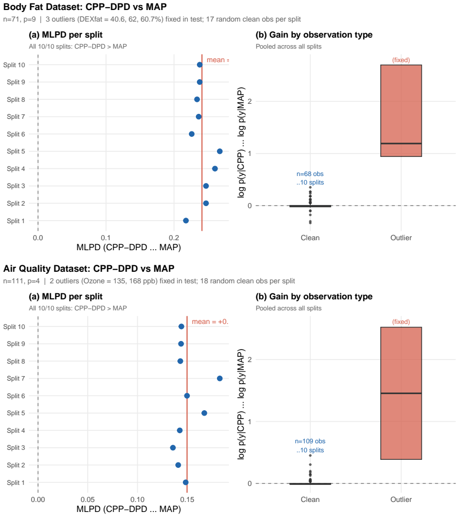
Finite-sample simulations confirm lower variance and better robustness than plug-in alternatives across contamination levels and dimensions.

Where Pith is reading between the lines

These are editorial extensions of the paper, not claims the author makes directly.

The distributional conformity idea may extend to other Bayesian models once leave-one-out predictives can be approximated.
The bounded-influence property suggests CPP could serve as a drop-in replacement for plug-in methods in settings where robustness to outliers is required.
Because the framework specializes cleanly when the posterior mean is linear, it supplies an immediate robust alternative for Gaussian process regression and spline models.

Load-bearing premise

The leave-one-out and swapped predictive distributions must be available in closed form and the swapped predictive mean must be differentiable in the candidate value.

What would settle it

A Monte Carlo experiment under an epsilon-contamination model in which the asymptotic variance of the CPP predictor exceeds that of a plug-in predictor with unbounded influence would refute the domination claim.

Figures

Figures reproduced from arXiv: 2605.24601 by Arkaprava Roy, Malay Ghosh.

read the original abstract

We propose a general robust prediction framework, termed conformal-projective prediction (CPP), that integrates Bayesian predictive modeling with ideas from conformal prediction. Rather than assessing conformity through residual-based scores, the CPP criterion defines conformity distributionally: a candidate value for a future response is considered conforming to the extent that its inclusion in the data leaves the leave-one-out predictive distributions of the observed responses undisturbed. The framework requires only that the leave-one-out and swapped predictive distributions are available in closed form and that the swapped predictive mean is differentiable in the candidate value. Under these conditions, we establish a general bounded-influence proposition and a general local convexity lemma, and prove that CPP dominates any plug-in predictor with unbounded influence in asymptotic variance under $\epsilon$-contamination models. When the posterior mean is linear in the observations, as in Gaussian linear models, basis-expansion regression, and Gaussian process regression, the swapped predictive mean is affine in the candidate value, yielding closed-form or one-dimensional optimization solutions and an efficient rank-two computational update; all general theoretical results specialize to explicit corollaries in this setting. Simulation experiments and two data analyses under the Gaussian linear model illustrate the finite-sample advantages of the proposed method, confirming the theoretical predictions across contamination levels, sample sizes, and predictor dimensions.

Editorial analysis

A structured set of objections, weighed in public.

Desk editor's note, referee report, simulated authors' rebuttal, and a circularity audit. Tearing a paper down is the easy half of reading it; the pith above is the substance, this is the friction.

Desk Editor's Note private letter to a colleague

The paper's main contribution is a distributional conformity score based on leave-one-out predictive stability that yields asymptotic dominance over unbounded-influence plug-ins under ε-contamination, but only when closed-form swapped predictives and differentiability hold.

read the letter

The new element here is the shift from residual scores to a distributional conformity criterion: a candidate y* is conforming if adding it leaves the leave-one-out predictives of the observed data essentially unchanged. From that they derive a bounded-influence result and show that the resulting predictor has lower asymptotic variance than any plug-in with unbounded influence under contamination, at least when the posterior mean is linear.

That dominance claim is the clearest payoff. The paper also works out the linear case (Gaussian linear models, basis expansions, GPR) in detail, where the swapped mean is affine, everything stays closed form, and rank-two updates make it practical. The simulations line up with the theory across contamination levels and dimensions.

The limitation is explicit in the setup: the general propositions require that leave-one-out and swapped predictives exist in closed form and that the swapped mean is differentiable in the candidate value. Once those are granted, the results follow, but the framework does not apply to models where those quantities are only available numerically or approximately. All the concrete corollaries and the reported experiments stay inside the linear-Gaussian setting, so we do not yet see how the method behaves when those conditions are relaxed.

The math appears internally consistent under the stated assumptions, with no obvious circularity. The citation pattern is standard for the area.

This is worth sending to referees. Readers working on robust Bayesian prediction or conformal methods will find the distributional criterion and the dominance result useful to engage with, even if they ultimately need to adapt the conditions. The paper is narrow enough that it will not change practice outside linear models, but the core idea is worth checking.

Referee Report

2 major / 2 minor

Summary. The paper proposes conformal-projective prediction (CPP), a robust Bayesian prediction framework that defines conformity distributionally via the effect of a candidate future response on leave-one-out predictive distributions of observed responses. It requires only closed-form availability of leave-one-out and swapped predictive distributions plus differentiability of the swapped predictive mean. Under these conditions the manuscript establishes a general bounded-influence proposition, a local convexity lemma, and proves that CPP dominates any plug-in predictor with unbounded influence in asymptotic variance under ε-contamination models. All results specialize explicitly to the linear posterior-mean case (Gaussian linear models, basis expansion, GPR), where the swapped mean is affine, yielding closed-form or one-dimensional optimization and rank-two updates. Finite-sample advantages are illustrated via simulations and two data analyses under the Gaussian linear model.

Significance. If the stated conditions hold and the derivations are correct, the work supplies a principled route to bounded-influence robust prediction inside standard Bayesian models, together with explicit dominance guarantees under ε-contamination and computationally efficient specializations. The explicit conditioning on closed-form LOO/swapped quantities and the rank-two update structure constitute clear strengths that facilitate immediate application in Gaussian linear and Gaussian-process settings.

major comments (2)

[Dominance result under ε-contamination models] The dominance claim (abstract) is load-bearing for the central contribution yet is conditioned on the swapped predictive mean being differentiable in the candidate value; the manuscript should verify that this differentiability is preserved under the ε-contamination model used in the asymptotic-variance comparison, or state the precise regularity needed to pass from the general proposition to the linear-case corollary.
[Local convexity lemma] The local convexity lemma is invoked to support the optimization procedure in the linear case, but the manuscript does not indicate whether the lemma continues to hold when the contamination fraction ε approaches the breakdown point of the underlying posterior; a brief remark on the range of ε for which convexity is guaranteed would strengthen the finite-sample claims.

minor comments (2)

[Abstract] The abstract states that simulations confirm theoretical predictions 'across contamination levels, sample sizes, and predictor dimensions,' yet provides no numerical ranges; adding these ranges would allow readers to assess the scope of the reported confirmation.
[Linear posterior-mean specialization] The rank-two computational update is described as efficient, but the manuscript does not compare its flop count or numerical stability against a naïve recomputation of the swapped predictive distribution; a short complexity remark would clarify the practical advantage.

Simulated Author's Rebuttal

2 responses · 0 unresolved

We thank the referee for the constructive comments and the recommendation of minor revision. We address the two major comments below.

read point-by-point responses

Referee: [Dominance result under ε-contamination models] The dominance claim (abstract) is load-bearing for the central contribution yet is conditioned on the swapped predictive mean being differentiable in the candidate value; the manuscript should verify that this differentiability is preserved under the ε-contamination model used in the asymptotic-variance comparison, or state the precise regularity needed to pass from the general proposition to the linear-case corollary.

Authors: In the linear posterior-mean specialization (Section 3), the swapped predictive mean is affine in the candidate value by the explicit form of the Gaussian linear posterior (see Equation (12)). Affine functions are differentiable everywhere. This structural property is a direct consequence of the linearity assumption on the posterior mean and therefore holds for any data-generating process, including data drawn from the ε-contamination model. No additional regularity conditions are required to apply the general bounded-influence proposition in the linear case. We will add a clarifying sentence to this effect immediately after the statement of the linear-case corollary. revision: yes
Referee: [Local convexity lemma] The local convexity lemma is invoked to support the optimization procedure in the linear case, but the manuscript does not indicate whether the lemma continues to hold when the contamination fraction ε approaches the breakdown point of the underlying posterior; a brief remark on the range of ε for which convexity is guaranteed would strengthen the finite-sample claims.

Authors: The local convexity lemma is derived solely from the maintained assumptions (closed-form LOO and swapped distributions together with differentiability of the swapped mean) and does not depend on the value of ε. In the Gaussian linear model the posterior remains Gaussian and the swapped mean remains affine for every ε ∈ [0,1). Consequently the lemma holds throughout this interval. We will insert a short remark stating that convexity is guaranteed for all contamination levels at which the model posterior is defined, which is the entire range ε < 1 under the linear Gaussian assumptions. This addition will strengthen the finite-sample discussion as suggested. revision: yes

Circularity Check

0 steps flagged

No significant circularity; derivation self-contained under stated assumptions

full rationale

The paper's core results (bounded-influence proposition, local convexity lemma, and ε-contamination dominance) are explicitly conditioned on the availability of closed-form leave-one-out/swapped predictive distributions and differentiability of the swapped mean. These are treated as modeling assumptions rather than derived quantities, and the dominance claim is proven only for the linear posterior-mean case (Gaussian linear models, etc.) where the assumptions hold by construction of the model class. No self-definitional steps, fitted inputs renamed as predictions, or load-bearing self-citations appear in the provided text; the framework does not reduce any claimed prediction to its own inputs by definition. The derivation chain therefore remains independent of the target results.

Axiom & Free-Parameter Ledger

0 free parameters · 0 axioms · 0 invented entities

Abstract-only review provides no explicit free parameters, axioms, or invented entities; cannot audit beyond the stated requirements for closed-form distributions and differentiability.

pith-pipeline@v0.9.1-grok · 5748 in / 936 out tokens · 25134 ms · 2026-06-30T13:12:51.174003+00:00 · methodology

discussion (0)

Reference graph

Works this paper leans on

11 extracted references · 1 canonical work pages

[1]

Vladimir Vovk, Alexander Gammerman, and Glenn Shafer.Algorithmic Learning in a Ran- dom World

doi: 10.1007/s11222-016-9696-4. Vladimir Vovk, Alexander Gammerman, and Glenn Shafer.Algorithmic Learning in a Ran- dom World. Springer, New York, 2005. Vladimir Vovk, Jieli Shen, Valery Manokhin, and Min-ge Xie. Nonparametric predictive distributions based on conformal prediction.Machine Learning, 108(3):445–474, 2019. doi: 10.1007/s10994-018-5755-8. Con...

work page doi:10.1007/s11222-016-9696-4 2005
[2]

The same domination condition gives the uniform law of large numbers sup a∈Uδ |Ψ′ n(a) +I(a)| p − →0

=|A|>0 by (A1). The same domination condition gives the uniform law of large numbers sup a∈Uδ |Ψ′ n(a) +I(a)| p − →0. Letλ= 1 4 I(a ∗ 0)>0. By the WLLN applied to−∂ aψ(Y;a ∗ 0),λ n := 1 4 |Ψ′ n(a∗ 0)| p − →λ. Chooseδ >0 small enough that onU δ = [a∗ 0 −δ, a ∗ 0 +δ]:|I(a)− I(a ∗ 0)|< 1 2 λby continuity ofI, and sup a∈Uδ |Ψ′ n(a) +I(a)|> 1 4 λwith probabili...
[3]

By the Inverse Function Theorem, with probability tending to 1, Ψ n is 1-to-1 onU δ and its image contains the interval around Ψ n(a∗

+I(a ∗ 0)| ≤ 1 4 λ+ 1 2 λ+ 1 4 λ=λ. By the Inverse Function Theorem, with probability tending to 1, Ψ n is 1-to-1 onU δ and its image contains the interval around Ψ n(a∗
[4]

SinceE[ψ(Y;a ∗ 0)] = 0 (asa ∗ 0 solves Ψ(a) = 0), the WLLN gives|Ψ n(a∗ 0)|< 1 2 λnδwith probability tending to 1, so 0∈Ψ n(Uδ) and the rootban = Ψ−1 n (0)∈U δ exists

with half-lengthλ nδ. SinceE[ψ(Y;a ∗ 0)] = 0 (asa ∗ 0 solves Ψ(a) = 0), the WLLN gives|Ψ n(a∗ 0)|< 1 2 λnδwith probability tending to 1, so 0∈Ψ n(Uδ) and the rootban = Ψ−1 n (0)∈U δ exists. Sinceδis arbitrary,ba n p − →a∗
[5]

For the asymptotic distribution, the mean-value expansion 0 = Ψn(a∗

Uniqueness in the sense of Huzurbazar [1948] follows from the 1-to-1 property. For the asymptotic distribution, the mean-value expansion 0 = Ψn(a∗

1948
[6]

+ (ban −a ∗ 0)Ψ′ n(˜an) gives √n(ban −a ∗
[7]

By (A3) and the CLT, √nΨ n(a∗ 0) d − →N(0, B)

=− √nΨ n(a∗ 0) Ψ′ n(˜an) . By (A3) and the CLT, √nΨ n(a∗ 0) d − →N(0, B). Sinceban p − →a∗ 0, we have ˜an p − →a∗ 0, and the uniform convergence established above gives Ψ′ n(˜an) p − → −I(a∗
[8]

Slutsky’s theorem gives√n(ban −a ∗ 0) d − →N(0, B/A2)

=A. Slutsky’s theorem gives√n(ban −a ∗ 0) d − →N(0, B/A2). A.2 Proof of Proposition 3 The first claim avar(a ∗ n) =B/A 2 follows directly from Proposition 2. The second claim avar(ˆfn(xn+1)) =V 0 holds by assumption on the plug-in predictor. For the Gaussian linear model with OLS plug-in,V 0 =x T n+1Σβxn+1 by the delta method applied tog(β) =x T n+1β (Cor...
[9]

On the event sup a |Jn(a)−J(a)|< η,J n(a∗ 0)≤J(a ∗

+ 3η. On the event sup a |Jn(a)−J(a)|< η,J n(a∗ 0)≤J(a ∗
[10]

+η, while for|a−a ∗ 0| ≥ε, Jn(a)≥J(a ∗
[11]

Hencea ∗ n cannot lie outside theε-ball arounda ∗ 0, giving P(|a∗ n −a ∗ 0| ≥ε)→0

+ 2η > J n(a∗ 0). Hencea ∗ n cannot lie outside theε-ball arounda ∗ 0, giving P(|a∗ n −a ∗ 0| ≥ε)→0. Under correct specification,a ∗ 0 =m 0, and consistencya ∗ n p − →m0 follows. A.6 Proof of Proposition 6 Posterior concentration of Π n atσ 2 ϵ and continuity ofJ(a;σ 2) implyQ n(a)→J(a;σ 2 ϵ ) uniformly overA; the argmin theorem givesa ∗ n →a ∗ ϵ. For the...

[1] [1]

Vladimir Vovk, Alexander Gammerman, and Glenn Shafer.Algorithmic Learning in a Ran- dom World

doi: 10.1007/s11222-016-9696-4. Vladimir Vovk, Alexander Gammerman, and Glenn Shafer.Algorithmic Learning in a Ran- dom World. Springer, New York, 2005. Vladimir Vovk, Jieli Shen, Valery Manokhin, and Min-ge Xie. Nonparametric predictive distributions based on conformal prediction.Machine Learning, 108(3):445–474, 2019. doi: 10.1007/s10994-018-5755-8. Con...

work page doi:10.1007/s11222-016-9696-4 2005

[2] [2]

The same domination condition gives the uniform law of large numbers sup a∈Uδ |Ψ′ n(a) +I(a)| p − →0

=|A|>0 by (A1). The same domination condition gives the uniform law of large numbers sup a∈Uδ |Ψ′ n(a) +I(a)| p − →0. Letλ= 1 4 I(a ∗ 0)>0. By the WLLN applied to−∂ aψ(Y;a ∗ 0),λ n := 1 4 |Ψ′ n(a∗ 0)| p − →λ. Chooseδ >0 small enough that onU δ = [a∗ 0 −δ, a ∗ 0 +δ]:|I(a)− I(a ∗ 0)|< 1 2 λby continuity ofI, and sup a∈Uδ |Ψ′ n(a) +I(a)|> 1 4 λwith probabili...

[3] [3]

By the Inverse Function Theorem, with probability tending to 1, Ψ n is 1-to-1 onU δ and its image contains the interval around Ψ n(a∗

+I(a ∗ 0)| ≤ 1 4 λ+ 1 2 λ+ 1 4 λ=λ. By the Inverse Function Theorem, with probability tending to 1, Ψ n is 1-to-1 onU δ and its image contains the interval around Ψ n(a∗

[4] [4]

SinceE[ψ(Y;a ∗ 0)] = 0 (asa ∗ 0 solves Ψ(a) = 0), the WLLN gives|Ψ n(a∗ 0)|< 1 2 λnδwith probability tending to 1, so 0∈Ψ n(Uδ) and the rootban = Ψ−1 n (0)∈U δ exists

with half-lengthλ nδ. SinceE[ψ(Y;a ∗ 0)] = 0 (asa ∗ 0 solves Ψ(a) = 0), the WLLN gives|Ψ n(a∗ 0)|< 1 2 λnδwith probability tending to 1, so 0∈Ψ n(Uδ) and the rootban = Ψ−1 n (0)∈U δ exists. Sinceδis arbitrary,ba n p − →a∗

[5] [5]

For the asymptotic distribution, the mean-value expansion 0 = Ψn(a∗

Uniqueness in the sense of Huzurbazar [1948] follows from the 1-to-1 property. For the asymptotic distribution, the mean-value expansion 0 = Ψn(a∗

1948

[6] [6]

+ (ban −a ∗ 0)Ψ′ n(˜an) gives √n(ban −a ∗

[7] [7]

By (A3) and the CLT, √nΨ n(a∗ 0) d − →N(0, B)

=− √nΨ n(a∗ 0) Ψ′ n(˜an) . By (A3) and the CLT, √nΨ n(a∗ 0) d − →N(0, B). Sinceban p − →a∗ 0, we have ˜an p − →a∗ 0, and the uniform convergence established above gives Ψ′ n(˜an) p − → −I(a∗

[8] [8]

Slutsky’s theorem gives√n(ban −a ∗ 0) d − →N(0, B/A2)

=A. Slutsky’s theorem gives√n(ban −a ∗ 0) d − →N(0, B/A2). A.2 Proof of Proposition 3 The first claim avar(a ∗ n) =B/A 2 follows directly from Proposition 2. The second claim avar(ˆfn(xn+1)) =V 0 holds by assumption on the plug-in predictor. For the Gaussian linear model with OLS plug-in,V 0 =x T n+1Σβxn+1 by the delta method applied tog(β) =x T n+1β (Cor...

[9] [9]

On the event sup a |Jn(a)−J(a)|< η,J n(a∗ 0)≤J(a ∗

+ 3η. On the event sup a |Jn(a)−J(a)|< η,J n(a∗ 0)≤J(a ∗

[10] [10]

+η, while for|a−a ∗ 0| ≥ε, Jn(a)≥J(a ∗

[11] [11]

Hencea ∗ n cannot lie outside theε-ball arounda ∗ 0, giving P(|a∗ n −a ∗ 0| ≥ε)→0

+ 2η > J n(a∗ 0). Hencea ∗ n cannot lie outside theε-ball arounda ∗ 0, giving P(|a∗ n −a ∗ 0| ≥ε)→0. Under correct specification,a ∗ 0 =m 0, and consistencya ∗ n p − →m0 follows. A.6 Proof of Proposition 6 Posterior concentration of Π n atσ 2 ϵ and continuity ofJ(a;σ 2) implyQ n(a)→J(a;σ 2 ϵ ) uniformly overA; the argmin theorem givesa ∗ n →a ∗ ϵ. For the...