Riemannian-Manifold Steering: Geometry-Aware Generative Autoencoders for Label-Free Steering
Pith reviewed 2026-06-30 11:54 UTC · model grok-4.3
The pith
Steering language models reduces to Riemannian geodesic computation on activation space using a learned output-distance metric.
A machine-rendered reading of the paper's core claim, the machinery that carries it, and where it could break.
Core claim
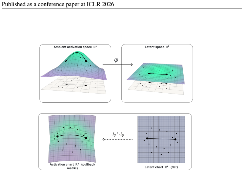
Manifold steering is recast as Riemannian geodesic computation on activation space, recovering linear and labelled-spline steering as geodesics under particular choices of metric. A principled metric is the output-space Hellinger distance pulled back to activations and approximated by a learned encoder trained on output distances over a small concept-token schema. The resulting label-free method drives the model onto the target class across all tasks in a standard four-task language-model arithmetic benchmark while following more behaviourally natural trajectories than baselines on smaller output spaces.
What carries the argument
Riemannian geodesic computation on activation space with the output-space Hellinger distance pulled back via a learned encoder on a concept-token schema.
If this is right
- Linear interpolation and labelled-spline steering emerge as geodesics under specific metric choices.
- The method steers models to target classes without per-prompt labels, topology priors, or per-task curve fitting.
- It produces more behaviourally natural trajectories than baselines on smaller output spaces.
- A single unified Riemannian framework covers existing manifold steering constructions.
- The encoder approximation operates on a small concept-token schema yet generalizes across the four-task benchmark.
Where Pith is reading between the lines
- The same encoder-based pullback could be tested on non-language generative models to check whether output distances remain informative in other domains.
- If the concept schema is expanded, the method might support steering without any task-specific data collection.
- Activation-space geodesics learned this way may offer a route to compare how different models represent the same output distinctions.
- Direct measurement of output Hellinger distances on larger models would test whether the encoder approximation remains necessary or becomes exact.
Load-bearing premise
The learned encoder trained on output distances over a small concept-token schema accurately approximates the pullback of the output-space Hellinger distance to activation space.
What would settle it
On a held-out arithmetic task the steered activations fail to produce outputs in the target class or produce trajectories that match baseline unnaturalness.
Figures
read the original abstract
Steering a language model - intervening on its internal activations to change downstream behaviour - has recently expanded beyond linear interpolation to nonlinear methods such as angular and kernelized steering, which define intervention transformations without learning an explicit geometry over paths in activation space. Freshly introduced geometry-aware manifold methods do learn such a geometry, but require labelled class centroids together with prescribed cyclic or sequential structure. These assumptions restrict where manifold steering can be applied, since existing constructions require labelled centroids and compatible boundary conditions. We recast manifold steering more broadly as \textbf{Riemannian geodesic computation} on activation space, recovering linear and labelled-spline steering as geodesics under particular choices of metric. A principled metric within this framework is the output-space Hellinger distance pulled back to activations; we approximate this with a learned encoder trained on output distances over a small concept-token schema - no per-prompt labels, no topology prior, and no per-task curve fitting. Empirically, the method reliably drives the model onto the target class across all tasks in a standard four-task language-model arithmetic benchmark, while following more behaviourally natural trajectories than baselines on smaller output spaces. We thereby provide a unified Riemannian framework for manifold steering together with a schema-supervised, label-free instantiation that operates without labelled centroids or prescribed boundary conditions.
Editorial analysis
A structured set of objections, weighed in public.
Referee Report
Summary. The paper recasts manifold steering of language models as Riemannian geodesic computation on activation space, recovering linear interpolation and labelled-spline methods as geodesics under special metrics. It identifies the pullback of output-space Hellinger distance as a principled metric and approximates it via a learned encoder trained on output distances over a small concept-token schema, enabling label-free operation without per-prompt labels, topology priors, or per-task curve fitting. The method is claimed to reliably steer models onto target classes across a standard four-task language-model arithmetic benchmark while producing more natural trajectories than baselines.
Significance. If the encoder approximation is shown to recover a metric close to the true Hellinger pullback, the work would supply a unified Riemannian framework that removes the labelled-centroid and boundary-condition requirements of prior manifold methods, broadening applicability. The empirical results on the four-task benchmark indicate practical utility for label-free steering, and the recovery of existing methods as special cases is a clear conceptual strength.
major comments (2)
- [Abstract] Abstract (paragraph on the principled metric and its approximation): the claim that the schema-trained encoder approximates the pullback of the output-space Hellinger distance is stated without a derivation showing that regression on output distances recovers the correct Riemannian structure on activations, nor any quantitative diagnostic (e.g., geodesic deviation or curvature comparison) measuring how close the induced metric remains to the true pullback when the activation map is nonlinear.
- [Empirical evaluation section] The central empirical claim (four-task benchmark success) rests on the unverified assumption that geodesics computed in the learned embedding yield steering trajectories that are geometrically meaningful with respect to the Hellinger metric; without an error bound or verification step, the Riemannian framing reduces to an empirical heuristic whose success does not confirm the geometric interpretation.
minor comments (2)
- [Method] Notation for the encoder and the pulled-back metric should be introduced with explicit symbols (e.g., define E and g_E) at first use to avoid ambiguity when comparing to the true pullback metric.
- [Experiments] The four-task benchmark description would benefit from a table listing the exact tasks, output spaces, and quantitative metrics (accuracy, trajectory naturalness) with error bars or multiple seeds.
Simulated Author's Rebuttal
We thank the referee for the careful reading and constructive comments on the geometric justification. We agree that the manuscript would be strengthened by an explicit derivation of the approximation and by verification diagnostics tying the learned geodesics to the Hellinger pullback. We address each point below and will revise accordingly.
read point-by-point responses
-
Referee: [Abstract] Abstract (paragraph on the principled metric and its approximation): the claim that the schema-trained encoder approximates the pullback of the output-space Hellinger distance is stated without a derivation showing that regression on output distances recovers the correct Riemannian structure on activations, nor any quantitative diagnostic (e.g., geodesic deviation or curvature comparison) measuring how close the induced metric remains to the true pullback when the activation map is nonlinear.
Authors: We acknowledge that the current text presents the distance-regression objective as an approximation without a formal derivation of how it recovers the Riemannian pullback structure, nor quantitative checks on the induced metric. In revision we will add a short theoretical paragraph deriving the approximation under the assumption that the encoder approximately preserves distances (i.e., learns a near-isometry), together with a practical diagnostic that compares geodesic lengths and endpoint Hellinger distances on a held-out activation subset. These additions will appear in the methods section. revision: yes
-
Referee: [Empirical evaluation section] The central empirical claim (four-task benchmark success) rests on the unverified assumption that geodesics computed in the learned embedding yield steering trajectories that are geometrically meaningful with respect to the Hellinger metric; without an error bound or verification step, the Riemannian framing reduces to an empirical heuristic whose success does not confirm the geometric interpretation.
Authors: We agree that the four-task results alone do not constitute a direct verification that the computed geodesics are close to true Hellinger geodesics. In the revision we will add a verification subsection that reports (i) the average Hellinger deviation of the steered outputs relative to the target class and (ii) a comparison of path lengths under the learned metric versus a direct output-space baseline on the same prompts. This will make the link between the Riemannian construction and the observed steering explicit while also stating the remaining approximation error. revision: yes
Circularity Check
No significant circularity detected
full rationale
The provided abstract frames the core construction as an approximation of the output-space Hellinger pullback metric via an encoder trained on distances from a fixed concept-token schema, then uses the resulting embedding for Riemannian geodesic steering. No equations, self-citations, or explicit reductions are present in the text that would make the steering result equivalent by construction to the encoder fit itself (e.g., no claim that the geodesics are forced to match the training distances or that the metric is defined circularly in terms of the output). The training step is described as schema-supervised and label-free for the target tasks, supplying independent content to the method rather than reducing the claimed Riemannian framework to a tautology. This is the most common honest finding for papers that introduce an approximation technique without asserting a closed derivation loop.
Axiom & Free-Parameter Ledger
free parameters (1)
- encoder parameters
axioms (1)
- domain assumption Activation space can be treated as a Riemannian manifold whose metric is the pullback of output-space Hellinger distance
Reference graph
Works this paper leans on
-
[1]
GAN Dissection: Visualizing and Understanding Generative Adversarial Networks
David Bau, Jun-Yan Zhu, Hendrik Strobelt, Bolei Zhou, Joshua B Tenenbaum, William T Freeman, and Antonio Torralba. Gan dissection: Visualizing and understanding generative adversarial networks.arXiv preprint arXiv:1811.10597,
work page internal anchor Pith review Pith/arXiv arXiv
-
[2]
ISBN 9780817634902. 17 Published as a conference paper at ICLR 2026 Nelson Elhage, Tristan Hume, Catherine Olsson, Nicholas Schiefer, Tom Henighan, Shauna Kravec, Zac Hatfield-Dodds, Robert Lasenby, Dawn Drain, Carol Chen, Roger Grosse, Sam McCan- dlish, Jared Kaplan, Dario Amodei, Martin Wattenberg, and Christopher Olah. Toy models of superposition,
2026
-
[3]
URLhttps://arxiv.org/abs/2209.10652. Joshua Engels, Eric J. Michaud, Isaac Liao, Wes Gurnee, and Max Tegmark. Not all language model features are one-dimensionally linear,
work page internal anchor Pith review Pith/arXiv arXiv
-
[4]
doi: 10.18653/v1/2024.acl-long.470
Association for Computational Linguistics. doi: 10.18653/v1/2024.acl-long.470. URLhttps://aclanthology.org/2024.acl-long.470/. Jürgen Jost.Riemannian Geometry and Geometric Analysis. Universitext. Springer,
-
[5]
mlr.press/v119/kalatzis20a.html
URL https://proceedings. mlr.press/v119/kalatzis20a.html. Subhash Kantamneni and Max Tegmark. Language models use trigonometry to do addition.arXiv preprint arXiv:2502.00873,
-
[6]
Inference-time intervention: Eliciting truthful answers from a language model.Advances in Neural Information Processing Systems, 36:41451–41530,
18 Published as a conference paper at ICLR 2026 Kenneth Li, Oam Patel, Fernanda Viégas, Hanspeter Pfister, and Martin Wattenberg. Inference-time intervention: Eliciting truthful answers from a language model.Advances in Neural Information Processing Systems, 36:41451–41530,
2026
-
[7]
UMAP: Uniform Manifold Approximation and Projection for Dimension Reduction
URLhttps://openreview.net/forum?id=aajyHYjjsk. Leland McInnes, John Healy, and James Melville. Umap: Uniform manifold approximation and projection for dimension reduction.arXiv preprint arXiv:1802.03426,
work page internal anchor Pith review Pith/arXiv arXiv
-
[8]
The Linear Representation Hypothesis and the Geometry of Large Language Models
Kiho Park, Yo Joong Choe, and Victor Veitch. The linear representation hypothesis and the geometry of large language models.arXiv preprint arXiv:2311.03658,
work page internal anchor Pith review Pith/arXiv arXiv
-
[9]
Shivam Raval, Hae Jin Song, Linlin Wu, Abir Harrasse, Jeff M
URL https: //arxiv.org/abs/2603.09972. Shivam Raval, Hae Jin Song, Linlin Wu, Abir Harrasse, Jeff M. Phillips, Fazl Barez, and Amirali Abdullah. Curveball steering: The right direction to steer isn’t always linear,
-
[10]
Nina Rimsky, Nick Gabrieli, Julian Schulz, Meg Tong, Evan Hubinger, and Alexander Turner
URL https://arxiv.org/abs/2603.09313. Nina Rimsky, Nick Gabrieli, Julian Schulz, Meg Tong, Evan Hubinger, and Alexander Turner. Steering llama 2 via contrastive activation addition. InProceedings of the 62nd Annual Meeting of the Association for Computational Linguistics (Volume 1: Long Papers), pp. 15504–15522,
-
[11]
Extracting latent steering vectors from pretrained language models
Nishant Subramani, Nivedita Suresh, and Matthew E Peters. Extracting latent steering vectors from pretrained language models. InFindings of the Association for Computational Linguistics: ACL 2022, pp. 566–581,
2022
- [12]
-
[13]
Steering Language Models With Activation Engineering
URL https://arxiv.org/abs/2308.10248. Laurens Van der Maaten and Geoffrey Hinton. Visualizing data using t-sne.Journal of machine learning research, 9(11),
work page internal anchor Pith review Pith/arXiv arXiv
-
[14]
pyvene: A library for understanding and improving PyTorch models via interventions
19 Published as a conference paper at ICLR 2026 Zhengxuan Wu, Atticus Geiger, Aryaman Arora, Jing Huang, Zheng Wang, Noah Goodman, Christo- pher Manning, and Christopher Potts. pyvene: A library for understanding and improving PyTorch models via interventions. In Kai-Wei Chang, Annie Lee, and Nazneen Rajani (eds.),Proceedings of the 2024 Conference of the...
2026
-
[15]
Manifold Steering Reveals the Shared Geometry of Neural Network Representation and Behavior
Association for Computational Linguistics. doi: 10.18653/v1/ 2024.naacl-demo.16. URLhttps://aclanthology.org/2024.naacl-demo.16/. Daniel Wurgaft, Can Rager, Matthew Kowal, Vasudev Shyam, Sheridan Feucht, Usha Bhalla, Tal Haklay, Eric Bigelow, Raphael Sarfati, Thomas McGrath, et al. Manifold steering reveals the shared geometry of neural network representa...
work page internal anchor Pith review Pith/arXiv arXiv doi:10.18653/v1/ 2024
-
[16]
20 Published as a conference paper at ICLR 2026 A METRIC AND SOLVER TAXONOMY TABLES For reference, we collect here the two taxonomy tables from the framework sections of the main text: table 6 enumerates the three metric instantiations (section 4), and table 7 the (metric, solver) cells we evaluate (section 5). Linear Labelled spline / GE on its image Lea...
2026
-
[17]
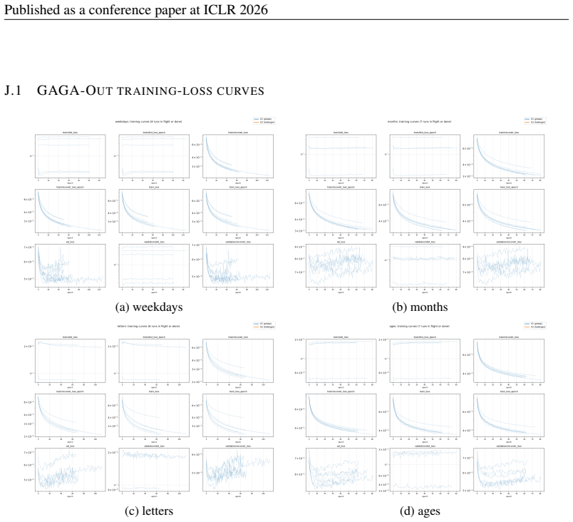
to standardize prompts and counterfactuals across tasks. For each of the four tasks (weekdays, months, letters, ages) the prompt template is the arithmetic formWhat is k {units} after z?, with k drawn uniformly from the task-specific support and z drawn from the conceptual domain Z. Per- task prompt counts (after a 5-paraphrase augmentation that increases...
2026
-
[18]
computed on the raw 4096-dimensional residual-stream activations. PHATE proceeds in three stages: (a) build a k-nearest-neighbor graph over the activations using Euclidean distance; (b) compute the random-walk transition matrix and raise it to a diffusion time t; (c) define the diffusion potential ϕi =−logP t i,· and take pairwise Euclidean distances betw...
2025
-
[19]
Differences from Sun et al. (2025).Three substantive deviations from the original GAGA: (1) wider hidden layers to accommodate the larger ambient dimension; (2) the cycle-consistency term described above; (3) PHATE / Hellinger distances are computed once and cached, rather than recomputed per epoch as in some GAGA variants for streaming data settings. We ...
2025
-
[20]
that an explicit G=J ⊤Jmatrix would require. We use the freeze-metric approximation: at each L-BFGS iteration, J(π k) is recomputed at the current waypoint butdetached from the optimizer’s computation graph(Arvanitidis et al., 2018). Gradients therefore flow only through the ∆k in the outer norm, not through the metric’s dependence on πk. This is the stan...
2018
-
[21]
(2026, Def
F.3 ANALYTICALJ F METRIC The metric specified in Wurgaft et al. (2026, Def. 1 eq
2026
-
[22]
We compute this metric exactly, with the following choices
is GF (h) =J F (h)⊤ gy JF (h) +ϵI, where F:A → Y is the rest-of-the-network forward map (layer-28 activations to output distribution restricted to the concept domain plus an “other” bin). We compute this metric exactly, with the following choices. 24 Published as a conference paper at ICLR 2026 Hellinger output coordinates make gy =I .We define F(h) = p s...
2026
-
[23]
(2026) can be recovered from eq
25 Published as a conference paper at ICLR 2026 F.6 SPLINE AS A DEGENERATE SPECIAL CASE The spline geodesic of Wurgaft et al. (2026) can be recovered from eq. (14) by (a) restricting π to the parametric spline family with control points at the labeled centroids; (b) replacing g with the metric implicitly induced by the spline’s path-length functional; (c)...
2026
-
[24]
reused as a reference, not re-run for this ablation. All numbers are mean across n= 21 pairs (weekdays) or n= 50 (months); paired-t compares each encoder’s GAGA path against the linear baseline (more negativet=more natural). Table 8: Weekdays: 15/15 PCA(64) encoder variants vs. the raw-4096 GAGA-Out reference. “pb_demap_r” is the Pearson correlation betwe...
-
[25]
encoder produces EBC within ∼10 −4 of the linear baseline, identical legibility (≈0.05 weekdays, ≈0.13 months), and identical endpoint target probability ( 0.049 weekdays, 0.128 months). The pb_demap_r column shows that several encoders do learn the supervision distance reasonably well (e.g. GAGA-PHATE λ=0.1 on weekdays at r= 0.69), but learning the dista...
-
[26]
Let D be the ambient activation dimension (D= 4096 ), K the number of path waypoints (K= 50 ), m the rank of the metric Jacobian (m≤ |Z|+ 1≪D ), and T the number of L-BFGS iterations. Write E for the cost of one encoder forward-or-backward pass, F for one forward-or-backward pass through the rest-of-network behaviour map F (only the ∼3-layer tail downstre...
2026
-
[27]
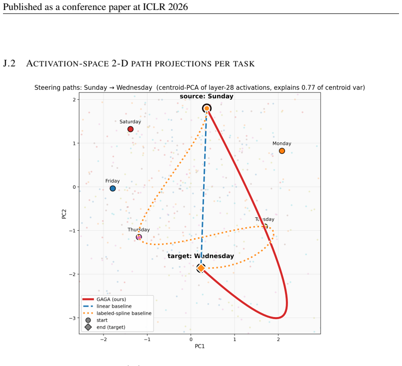
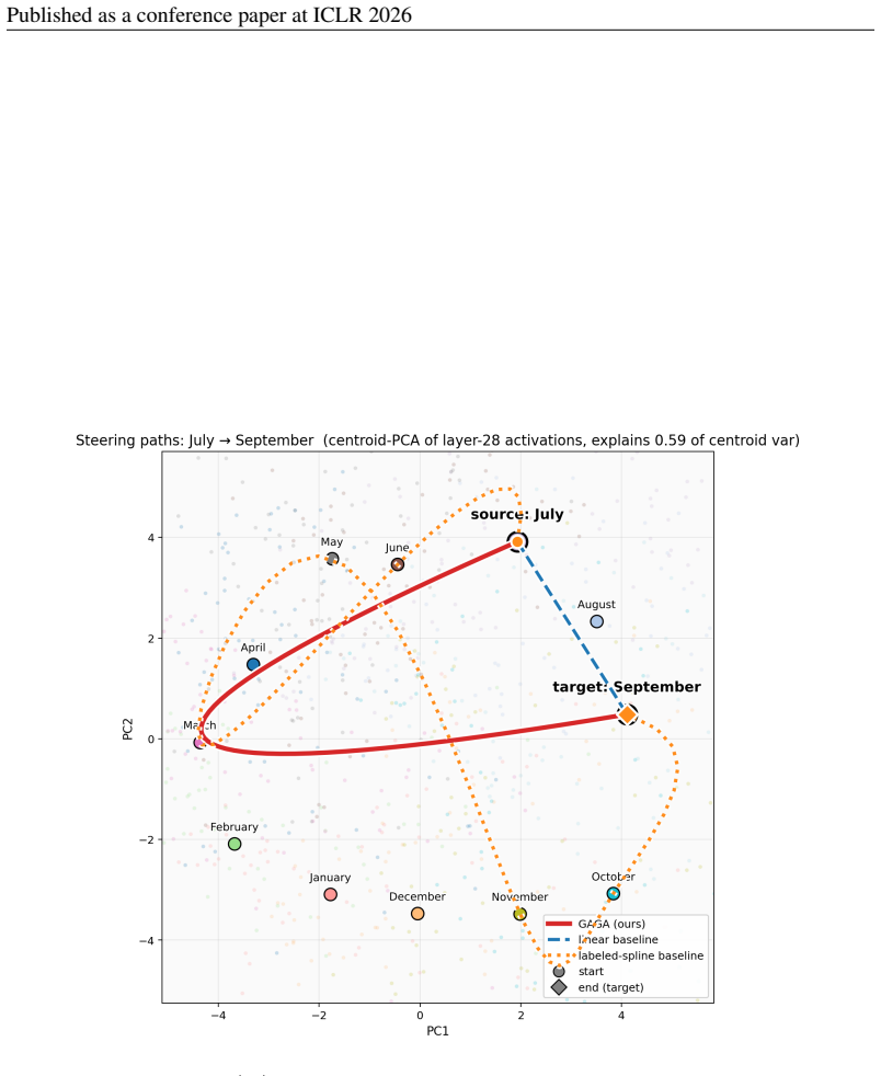
Background grey points are the training-prompt activations; coloured points mark per-class centroids
29 Published as a conference paper at ICLR 2026 J.2 ACTIVATION-SPACE2-DPATH PROJECTIONS PER TASK Figure 3:Weekdays(cyclic, |Z|= 7 ): activation-space paths for the example pair Sunday → Wednesday, projected onto the top two principal components of the per-prompt PCA(64) activations. Background grey points are the training-prompt activations; coloured poin...
2026
-
[28]
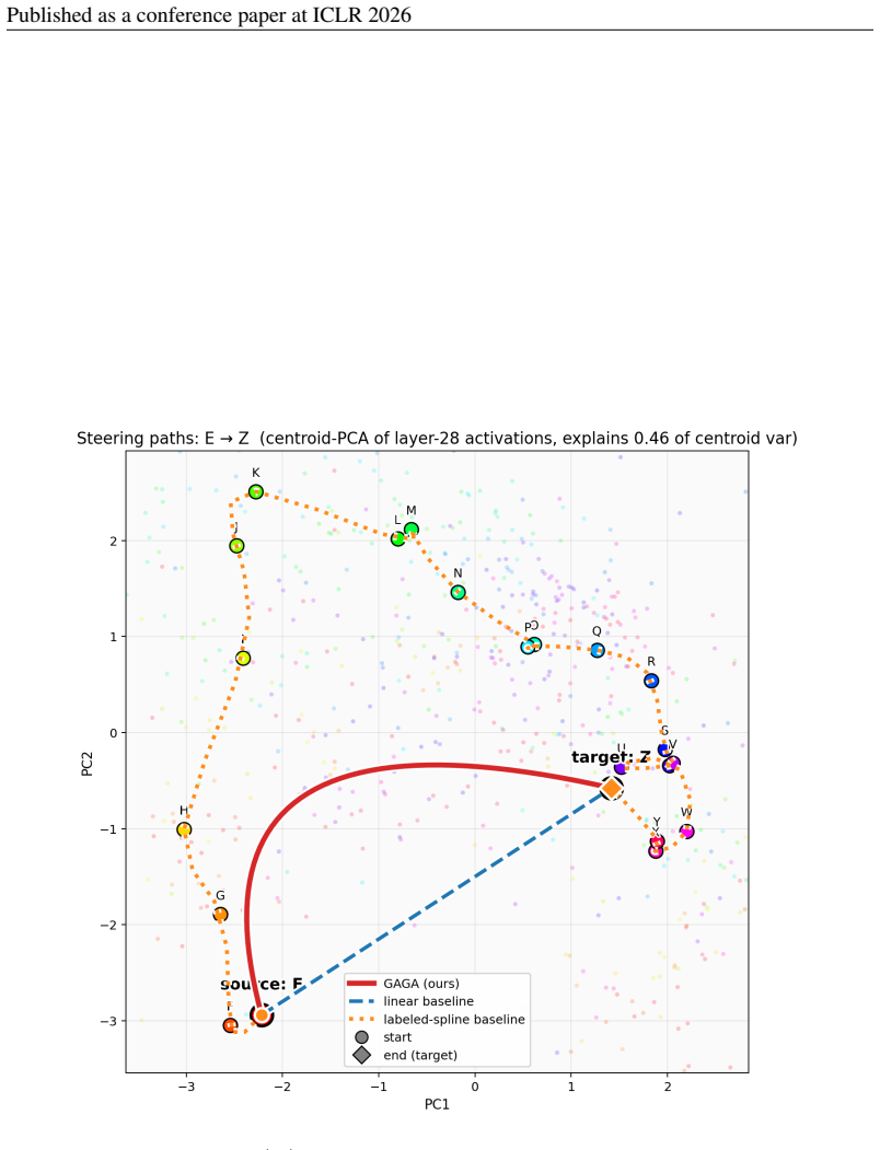
31 Published as a conference paper at ICLR 2026 Figure 5:Letters(sequential, |Z|= 22 ): activation-space paths for the longest sequential pair E→ Z
is a consequence of this aggressive curvature, not of better steering: the longer arc passes through low-density activation regions and produces unnaturally smeared output distributions in behavior space. 31 Published as a conference paper at ICLR 2026 Figure 5:Letters(sequential, |Z|= 22 ): activation-space paths for the longest sequential pair E→ Z. Sam...
2026
-
[29]
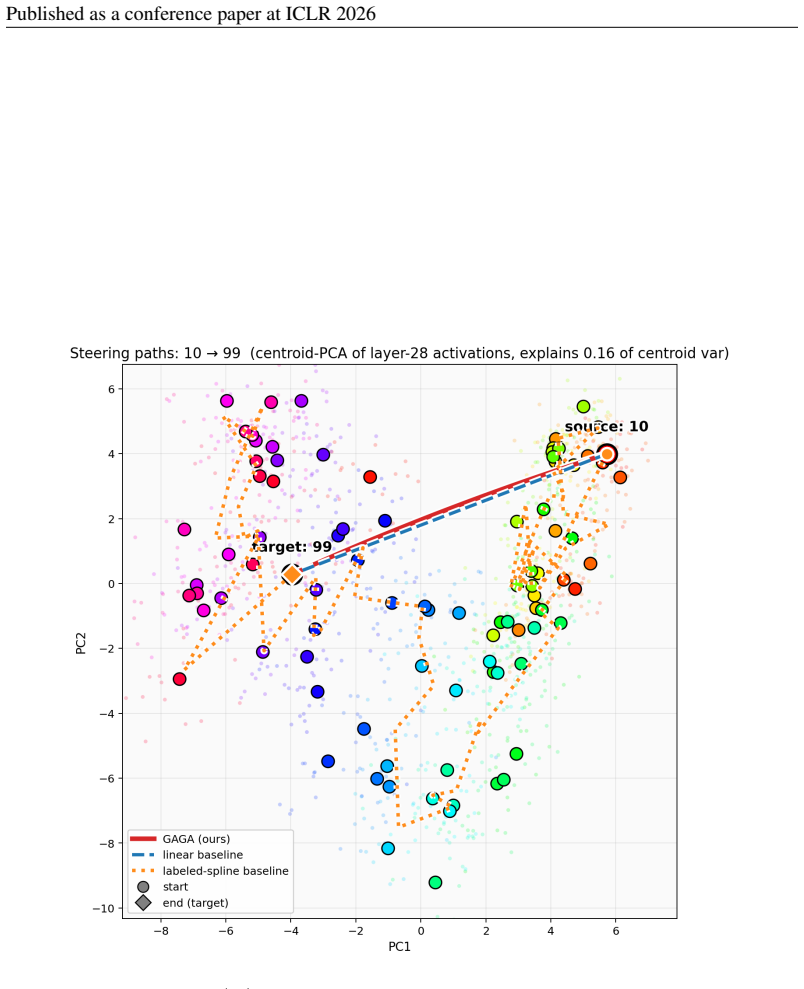
32 Published as a conference paper at ICLR 2026 Figure 6:Ages(sequential, |Z| ≈91 ): activation-space paths for the long-hop pair age-10→ age-99
With 22 well-separated sequential centroids, the labeled spline becomes a much longer curve and drifts further from the training-prompt cloud than on weekdays/months; GAGA’s geodesic stays close throughout. 32 Published as a conference paper at ICLR 2026 Figure 6:Ages(sequential, |Z| ≈91 ): activation-space paths for the long-hop pair age-10→ age-99. Same...
2026
-
[30]
, 99, which is why the labeled spline scores 95% on the visit-intermediates rate (table 4)
With∼91 sequential centroids, the labeled cubic spline curls dramatically through each centroid in order; in the 2-D projection shown here, the path visibly visits intermediate ages 10, 11, 12, . . ., 99, which is why the labeled spline scores 95% on the visit-intermediates rate (table 4). The cost: the spline’s behavior-space arc length is 8.13 on this t...
2026
-
[31]
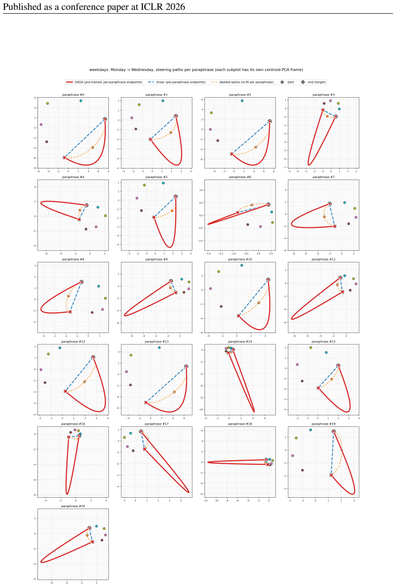
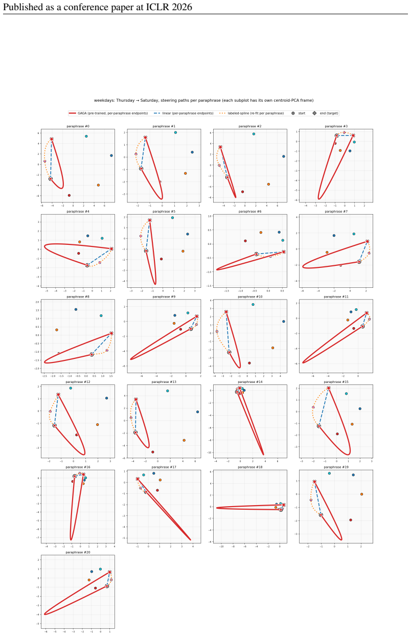
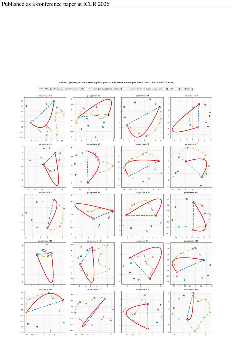
36 Published as a conference paper at ICLR 2026 Figure 9:Months, paraphrase consistency(January → July)
We include a second example pair to confirm the paraphrase-invariance behaviour is not specific to the Monday→Wednesday pair. 36 Published as a conference paper at ICLR 2026 Figure 9:Months, paraphrase consistency(January → July). Same conventions as fig. 7, on the months task. The longer cyclic shortest-path (six hops) magnifies inter-method differences:...
2026
-
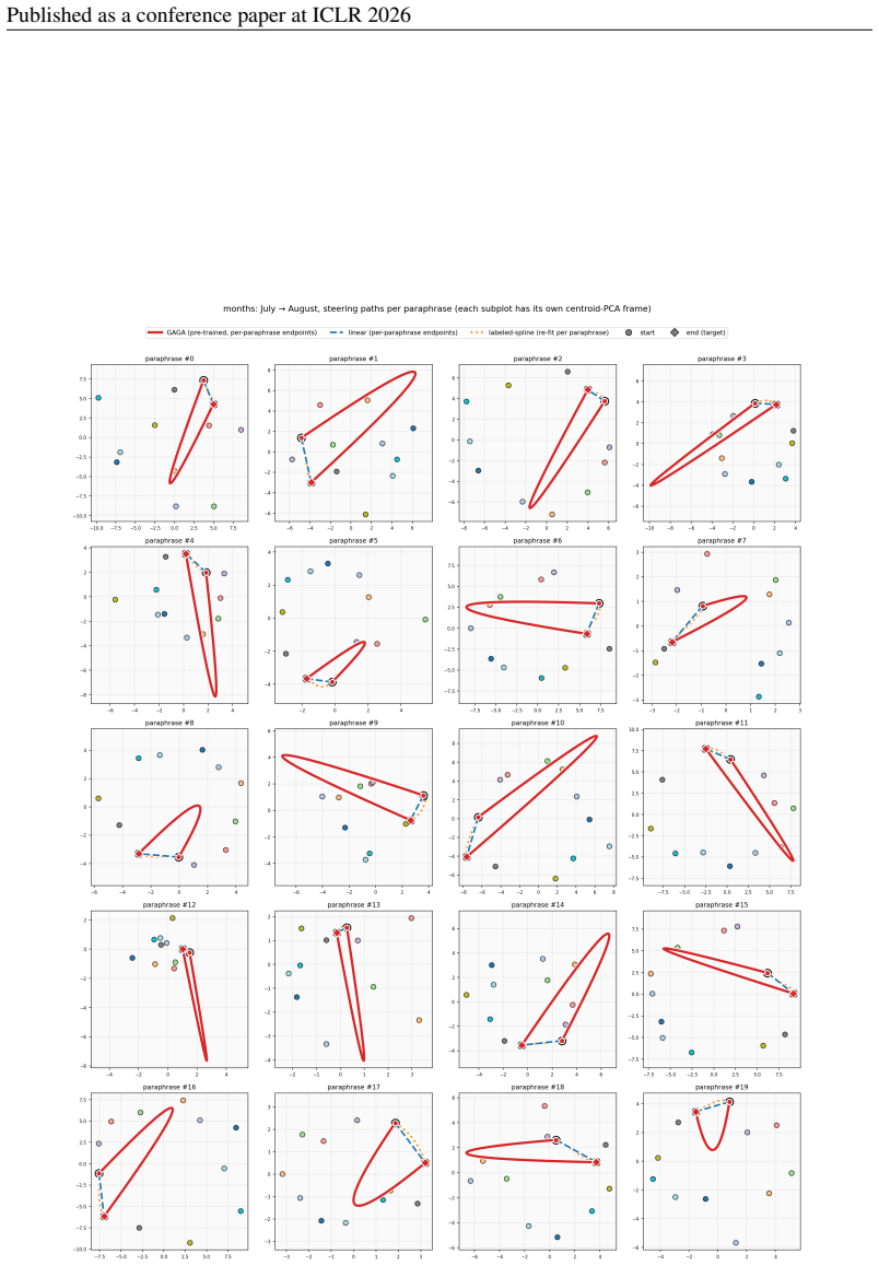
[32]
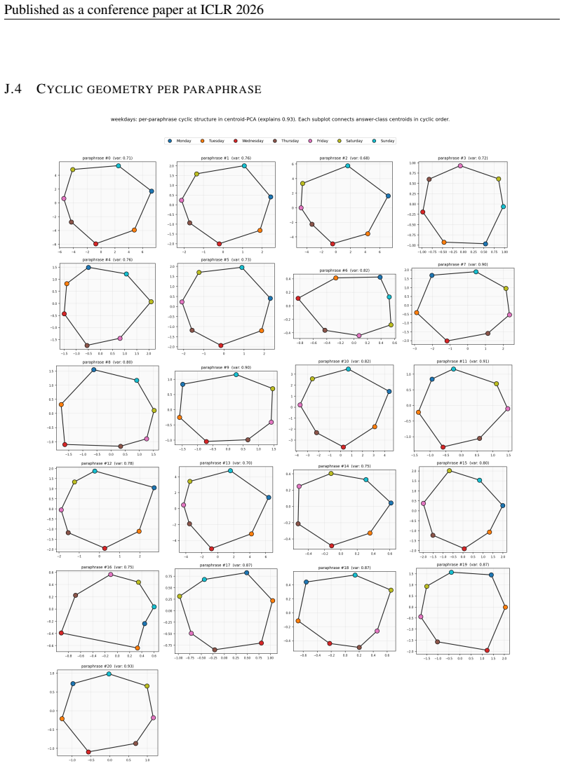
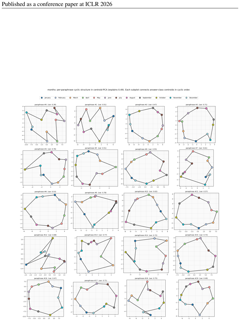
With only one cyclic hop the three methods are visually closer; even here the GAGA path is the tightest across paraphrases. 38 Published as a conference paper at ICLR 2026 J.4 CYCLIC GEOMETRY PER PARAPHRASE Figure 11:Weekdays, cyclic latent geometry per paraphrase.We plot the GAGA-PHATE latent (R2) embedding of training-prompt activations, coloured by gro...
2026
discussion (0)
Sign in with ORCID, Apple, or X to comment. Anyone can read and Pith papers without signing in.