REVIEW 2 major objections 1 minor 8 references
Reformulating zeroth-order terms into aligned constraints mitigates gradient conflicts in PINNs.
Reviewed by Pith at T0; open to challenge. T0 means a machine referee read the full paper against a public rubric. the ladder, T0–T4 →
T0 review · grok-4.3
2026-06-30 12:36 UTC pith:VJS6WXCH
load-bearing objection CAML reformulates boundary terms in PINNs for gradient alignment but the abstract shows no derivation that the new loss keeps the same solutions as the original BVP. the 2 major comments →
Mitigating Gradient Pathology in PINNs through Aligned Constraint
The pith
A machine-rendered reading of the paper's core claim, the machinery that carries it, and where it could break.
Core claim
The central claim is that gradient pathology in PINNs is caused by opposing gradients between PDE residuals and boundary constraints. Reformulating all zeroth-order terms into aligned constraints via Constraint-Aligned loss with Manifold Lifting effectively mitigates these conflicts, and introducing a delay factor helps the optimizer avoid high-curvature regions, resulting in enhanced numerical stability and efficiency for complex problems.
What carries the argument
Constraint-Aligned loss with Manifold Lifting (CAML), which reformulates zeroth-order terms as aligned constraints to eliminate gradient opposition.
Load-bearing premise
Gradient pathology stems mainly from opposing directions of PDE residual gradients and boundary constraint gradients, and reformulating the terms will align them without creating new optimization difficulties or reducing accuracy.
What would settle it
Running the CAML method on a known complex PDE where gradient directions remain opposing after reformulation, or where accuracy drops compared to baseline, would disprove the central claim.
If this is right
- Training of PINNs avoids local minima caused by gradient opposition between residuals and boundaries.
- Methods like adaptive weighting or geometry-limited hard constraints become unnecessary for many cases.
- Numerical stability and training efficiency improve significantly in highly complex PINN problems.
- The optimizer can skip high-curvature areas using the introduced delay factor.
Where Pith is reading between the lines
- This alignment strategy could apply to other neural network tasks where multiple loss terms conflict.
- Manifold lifting might offer a general way to handle constraint satisfaction in optimization without explicit enforcement.
- Further tests on time-dependent or high-dimensional PDEs would show if the benefits hold beyond the reported experiments.
Editorial analysis
A structured set of objections, weighed in public.
Referee Report
Summary. The manuscript claims that gradient pathology in PINNs is caused by opposing gradients from PDE residuals and boundary constraints. It proposes Constraint-Aligned loss with Manifold Lifting (CAML), which reformulates all zeroth-order terms into aligned constraints to mitigate conflicts, plus a delay factor to avoid high-curvature regions. The authors state that experiments show significantly improved numerical stability and efficiency on complex PINN problems, with code released openly.
Significance. If the reformulation is proven equivalent to the original BVP and the stability gains are demonstrated with quantitative metrics and baselines, the approach could offer a general technique for resolving ill-conditioning in PINN optimization across geometries. The open-sourced code is a strength for reproducibility.
major comments (2)
- [Method] The central claim requires that the aligned-constraint reformulation preserves the original BVP minimizer. No derivation establishing mathematical equivalence between the transformed loss and the original PDE+BC problem is provided (see the method description and any equations defining the manifold lifting or alignment enforcement).
- [Abstract / Experiments] The abstract asserts that 'experiments demonstrate that our CAML significantly enhances numerical stability and efficiency', yet supplies no quantitative metrics, baselines, problem specifications, error tables, or convergence plots. This absence prevents evaluation of whether the claimed gains are load-bearing for the stability conclusion.
minor comments (1)
- [Method] Notation for the delay factor and its integration into the optimizer is introduced without a clear algorithmic description or pseudocode.
Simulated Author's Rebuttal
We thank the referee for the constructive feedback. We address the two major comments point-by-point below.
read point-by-point responses
-
Referee: [Method] The central claim requires that the aligned-constraint reformulation preserves the original BVP minimizer. No derivation establishing mathematical equivalence between the transformed loss and the original PDE+BC problem is provided (see the method description and any equations defining the manifold lifting or alignment enforcement).
Authors: We agree that the manuscript lacks an explicit derivation establishing equivalence. In the revised version we will insert a dedicated subsection deriving that the manifold lifting and alignment operations preserve the original BVP minimizer, showing that the transformed loss shares the same critical points under the stated assumptions on the constraint functions. revision: yes
-
Referee: [Abstract / Experiments] The abstract asserts that 'experiments demonstrate that our CAML significantly enhances numerical stability and efficiency', yet supplies no quantitative metrics, baselines, problem specifications, error tables, or convergence plots. This absence prevents evaluation of whether the claimed gains are load-bearing for the stability conclusion.
Authors: The current abstract is deliberately concise. We will expand it to report the key quantitative metrics (error norms, iteration counts, stability indicators) and baseline comparisons already present in Section 4, while ensuring the experimental section contains the requested tables and plots with problem specifications. revision: yes
Circularity Check
No circularity detected; derivation chain self-contained with no reductions to inputs
full rationale
The abstract describes an analysis of gradient pathology in PINNs leading to the CAML method via reformulation of zeroth-order terms into aligned constraints, plus a delay factor. No equations, loss functions, or derivations are presented that could reduce a claimed prediction or result to a fitted parameter or self-citation by construction. No self-citations, uniqueness theorems, or ansatzes are invoked in the provided text. The central claim rests on empirical experiments rather than any load-bearing mathematical equivalence that collapses to the inputs. This matches the default expectation for non-circular papers.
Axiom & Free-Parameter Ledger
read the original abstract
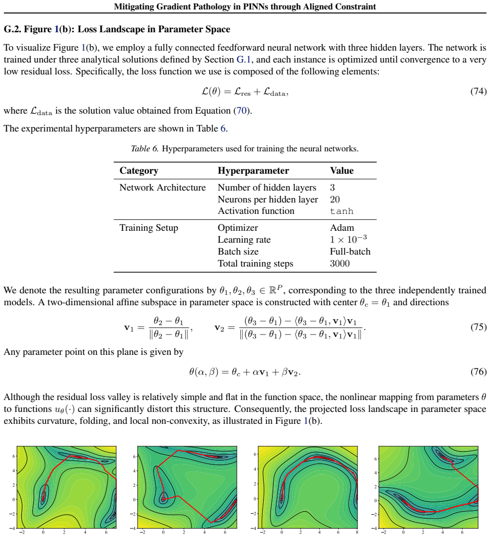
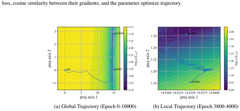
While Physics-Informed Neural Networks (PINNs) are powerful for solving Partial Differential Equations (PDEs), their training is often paralyzed by gradient pathology. The gradients from the PDE residuals and boundary constraints oppose each other, trapping the model in local minima. Current solutions, such as adaptive weighting or hard constraints, either fail to fundamentally resolve this ill-conditioning or are limited to simple geometries. In this study, we systematically analyze the possible causes of this gradient pathology from the perspectives of loss landscapes and optimization dynamics. Based on the obtained conclusion, we propose Constraint-Aligned loss with Manifold Lifting (CAML). By reformulating all zeroth-order terms into aligned constraints, our method effectively mitigates gradient conflicts. In addition, we introduce a delay factor to help the optimizer skip the high-curvature area. Experiments demonstrate that our CAML significantly enhances numerical stability and efficiency in highly complex PINN problems. Our code is open-sourced on https://github.com/YichenLuo-0/CAML.
Figures






Reference graph
Works this paper leans on
-
[1]
Neural operator: Graph kernel network for partial differential equations
Anandkumar, A., Azizzadenesheli, K., Bhattacharya, K., Kovachki, N., Li, Z., Liu, B., and Stuart, A. Neural operator: Graph kernel network for partial differential equations. InICLR 2020 Workshop on Integration of Deep Neural Models and Differential Equations,
work page 2020
-
[2]
Physics-Informed Transformer Networks
Dos Santos, F., Akhound-Sadegh, T., and Ravanbakhsh, S. Physics-Informed Transformer Networks. InNeurIPS 2023 Workshop on The Symbiosis of Deep Learning and Differential Equations III,
work page 2023
-
[3]
Workshop paper. Du, Y ., Czarnecki, W. M., Jayakumar, S. M., Farajtabar, M., Pascanu, R., and Lakshminarayanan, B. Adapting auxiliary losses using gradient similarity.arXiv preprint arXiv:1812.02224,
-
[4]
/uni00000013/uni00000015/uni00000013/uni00000013/uni00000013/uni00000017/uni00000013/uni00000013/uni00000013/uni00000019/uni00000013/uni00000013/uni00000013/uni0000001b/uni00000013/uni00000013/uni00000013/uni00000014/uni00000013/uni00000013/uni00000013/uni00000013 /uni00000048/uni00000053/uni00000052/uni00000046/uni0000004b /uni00000014/uni00000013/uni000...
work page 2000
-
[5]
The task is to solve for a scalar field u(x, y) governed by a variable-coefficient second-order elliptic equation with a reaction term. This benchmark tests models’ ability to handle spatially varying anisotropic operators and nontrivial domain geometries. Inside the domain,usatisfies a generalized Helmholtz equation of the form −∇ · A(x, y)∇u(x, y) +q(x,...
work page 2000
-
[6]
Table 15.The computational cost of CAML in linear PDEs. FP: the forward propagation process; AD: automatic differentiation of PDE residual and boundary conditions; AC: calculation of the additive constant c; BP: the backward propagation process; Percentage: The proportion of time spent on calculatingcin the total duration. FP ADACBP Percentage MLP Single ...
-
[7]
Table 16.The computational cost of CAML in non-linear PDEs. FP: the forward propagation process; AD: automatic differentiation of PDE residual and boundary conditions; AC: calculation of the additive constant c; BP: the backward propagation process; Percentage: The proportion of time spent on calculatingcin the total duration. FP ADACBP Percentage Kfew = ...
-
[8]
The definitions of Stp and L2 are consistent with those in the main experiment
Table 18.Sensitivity of CAML to the delay-residual schedule (td, tr) on the Poisson benchmark (MLP backbone). The definitions of Stp and L2 are consistent with those in the main experiment. Configurations that cannot achieve the expected accuracy within the maximum training budgetT max are indicated by ‘−’. td/tr 0/0 40/160 80/320 120/480 160/640 200/800 ...
work page 1984
discussion (0)
Sign in with ORCID, Apple, or X to comment. Anyone can read and Pith papers without signing in.