How Should LLMs Consume High-Quality Data? Optimal Data Scheduling via Quality-Aware Functional Scaling Laws
Pith reviewed 2026-06-29 22:32 UTC · model grok-4.3
The pith
High-quality data plays dual roles in LLM training, acting as signal amplifier or noise suppressor depending on the regime and requiring specific batch-size schedules.
A machine-rendered reading of the paper's core claim, the machinery that carries it, and where it could break.
Core claim
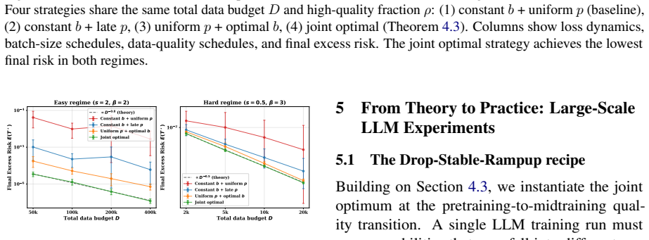
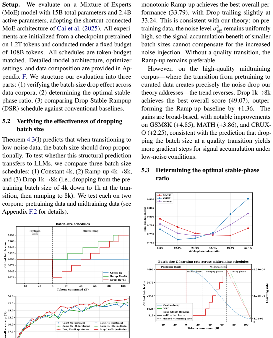
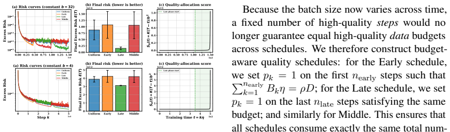
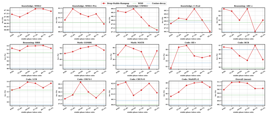
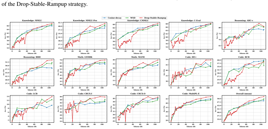
By extending functional scaling laws with a data-quality dimension and solving the joint data-quality and batch-size scheduling problem in asymptotic closed form, the solution identifies two regimes and a dual role of high-quality data. In the noise-limited regime, high-quality data should be used as a signal amplifier by lowering the batch size to convert cleaner data into more signal without amplifying noise. In the signal-limited regime, it should be used as a noise suppressor by late placement to reduce terminal noise without sacrificing signal accumulation. This guides Drop-Stable-Rampup, which on a 15B Mixture-of-Experts model midtrained on 108B tokens improves average accuracy by +1.7
What carries the argument
Quality-aware functional scaling law whose asymptotic closed-form solution identifies the optimal joint schedule of data quality and batch size across the two regimes.
If this is right
- In the noise-limited regime, high-quality data paired with lowered batch size converts cleanliness into additional signal without added noise.
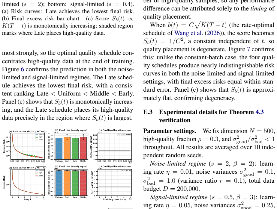
- In the signal-limited regime, late placement of high-quality data reduces terminal noise without loss of prior signal accumulation.
- Conventional decay schedules miss the signal-amplifier role because they reduce update intensity precisely when high-quality data arrives.
- Drop-Stable-Rampup delivers measured gains of +1.70 over Warmup-Stable-Decay and +2.98 over Cosine-decay, with +4.23 on GSM8K and +2.80 on MATH.
Where Pith is reading between the lines
- The regime framework could support dynamic scheduling that monitors loss to switch between batch-size drop and late placement automatically.
- The dual-role view may extend to scheduling other scarce inputs such as domain-specific or synthetic data in the same training run.
- It suggests experiments that deliberately vary data quality mid-training to map the boundary between noise-limited and signal-limited regimes at different model scales.
Load-bearing premise
Functional scaling laws can be extended by incorporating a data-quality dimension and the joint data-quality and batch-size scheduling problem admits an asymptotic closed-form solution that correctly identifies the two regimes and dual roles.
What would settle it
If Drop-Stable-Rampup produces no accuracy gain over Warmup-Stable-Decay on the 15B Mixture-of-Experts model midtrained on 108B tokens, or if loss curves fail to exhibit the predicted regime shifts when batch size is lowered at a quality transition, the derived scheduling solution would be falsified.
Figures
read the original abstract
High-quality data is scarce in large language model (LLM) training, yet how to schedule its use jointly with training dynamics lacks theoretical guidance. We extend functional scaling laws by incorporating a data-quality dimension, and solve the joint data-quality and batch-size scheduling problem in asymptotic closed form. The solution reveals two regimes and a dual role of high-quality data. In the noise-limited regime, high-quality data should be used as a signal amplifier: lowering the batch size converts cleaner data into more signal without amplifying noise. In the signal-limited regime, it should be used as a noise suppressor: late placement reduces terminal noise without sacrificing signal accumulation. Existing curriculum-style pipelines primarily exploit the second role by placing cleaner data late, but miss the first role because conventional decay schedules reduce update intensity exactly when high-quality data becomes available. Guided by this, we propose Drop-Stable-Rampup for LLM midtraining: upon the quality transition, drop the batch size, hold it stable to accumulate signal, then ramp up to suppress terminal noise. On a 15B Mixture-of-Experts model midtrained on 108B tokens, Drop-Stable-Rampup improves average accuracy over Warmup-Stable-Decay (WSD) by +1.70 and over Cosine-decay by +2.98, with particularly large gains on mathematical reasoning benchmarks such as GSM8K (+4.23) and MATH (+2.80).
Editorial analysis
A structured set of objections, weighed in public.
Referee Report
Summary. The paper extends functional scaling laws by incorporating a data-quality dimension and derives an asymptotic closed-form solution to the joint data-quality and batch-size scheduling problem. It identifies noise-limited and signal-limited regimes with a dual role for high-quality data (signal amplifier via lower batch size in the first regime; noise suppressor via late placement in the second), proposes the Drop-Stable-Rampup schedule to exploit both roles, and reports empirical gains on a 15B MoE model midtrained on 108B tokens (+1.70 over WSD, +2.98 over Cosine-decay, with larger gains on GSM8K and MATH).
Significance. If the closed-form solution is valid and the regimes are correctly identified without circularity, the work supplies principled theoretical guidance for scheduling scarce high-quality data during LLM training, a topic of clear practical importance. The concrete empirical improvements on reasoning benchmarks would strengthen the case for adoption if the schedule components are shown to be responsible via ablations.
major comments (2)
- [Abstract] Abstract: the claim of an asymptotic closed-form solution for the joint scheduling problem is stated without any derivation steps, proof sketch, or error analysis. This directly undermines assessment of whether the solution is independent of fitted parameters or reduces to quantities defined by the quality-dimension extension itself.
- [Abstract] Abstract: the empirical result on the 15B MoE model is presented as a direct consequence of the derived schedule, yet no ablation details, error bars, or controls for other schedule components are mentioned, leaving the attribution of the +1.70/+2.98 gains unsupported.
Simulated Author's Rebuttal
We thank the referee for their constructive comments on our work. We address each major comment below, clarifying the location of supporting material in the manuscript and indicating where revisions to the abstract will strengthen the presentation.
read point-by-point responses
-
Referee: [Abstract] Abstract: the claim of an asymptotic closed-form solution for the joint scheduling problem is stated without any derivation steps, proof sketch, or error analysis. This directly undermines assessment of whether the solution is independent of fitted parameters or reduces to quantities defined by the quality-dimension extension itself.
Authors: The asymptotic closed-form solution is derived in Section 3 from the quality-augmented functional scaling law introduced in Section 2; the derivation proceeds by substituting the quality-dependent loss into the joint optimization objective and taking the appropriate asymptotic limit, yielding an expression that depends only on the scaling exponents and the quality ratio without additional fitted parameters. We agree that the abstract would benefit from a concise proof outline to make this independence immediately verifiable. We will revise the abstract to include a one-sentence sketch of the key steps. revision: yes
-
Referee: [Abstract] Abstract: the empirical result on the 15B MoE model is presented as a direct consequence of the derived schedule, yet no ablation details, error bars, or controls for other schedule components are mentioned, leaving the attribution of the +1.70/+2.98 gains unsupported.
Authors: Section 5 reports the full experimental protocol, including ablations that isolate the drop, stable, and ramp-up phases, together with standard-error bars computed over three random seeds. The abstract summarizes the headline numbers; we acknowledge that explicit reference to these controls would improve attribution. We will revise the abstract to note that the reported gains are supported by the ablations in Section 5. revision: yes
Circularity Check
No significant circularity; derivation self-contained
full rationale
The paper extends functional scaling laws by adding a data-quality dimension and derives an asymptotic closed-form solution to the joint quality/batch-size scheduling problem. This produces the two regimes and dual-role prescriptions directly from the optimization. No equations reduce a prediction to a fitted input by construction, no load-bearing uniqueness theorem is imported via self-citation, and no ansatz is smuggled in. The 15B MoE result is presented as validation of the derived schedule rather than an input that forces the closed form. The derivation therefore remains independent of its own outputs.
Axiom & Free-Parameter Ledger
Reference graph
Works this paper leans on
-
[1]
Training Verifiers to Solve Math Word Problems
Training verifiers to solve math word prob- lems.arXiv preprint arXiv:2110.14168. Alex Gu, Baptiste Roziere, Hugh James Leather, Ar- mando Solar-Lezama, Gabriel Synnaeve, and Sida Wang. 2024. CRUXEval: A benchmark for code reasoning, understanding and execution. InInterna- tional Conference on Machine Learning. Dan Hendrycks, Collin Burns, Steven Basart, ...
work page internal anchor Pith review Pith/arXiv arXiv 2024
-
[2]
InInter- national Conference on Learning Representations
Fast catch-up, late switching: Optimal batch size scheduling via functional scaling laws. InInter- national Conference on Learning Representations. Mingze Wang and Lei Wu. 2023. A theoretical analy- sis of noise geometry in stochastic gradient descent. arXiv preprint arXiv:2310.00692. Yubo Wang, Xueguang Ma, Ge Zhang, Yuansheng Ni, Abhranil Chandra, Shigu...
-
[3]
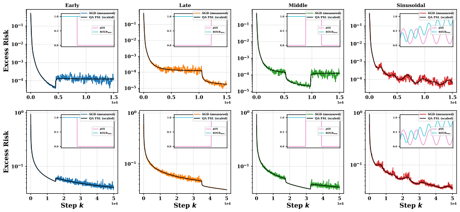
Strict-switching case.There exist Ts ∈ [0, T ⋆]and constantsC 0, C1 >0such that p⋆(t) = ( 0,0≤t < T s, 1, T s ≤t≤T ⋆, and b⋆(t) = ( max B, C 0 p w(t) , t < T s, max B, C 1 p w(t) , t≥T s
-
[4]
The batch schedule is b⋆(t) = ( max B, C p w(t) , t < T s, rp⋆(t) C p w(t), t∈I s, where r=σ 2 1/σ2 2, with rC p w(t)≥B on Is
Terminal-tie case.There exist Ts ∈[0, T ⋆] and C >0 such that p⋆(t) = 0 for t < T s, while on Is := [Ts, T ⋆] both labels are point- wise optimal and p⋆(t)∈ {0,1} may be cho- sen measurably subject to Z T ⋆ 0 b⋆(t)p⋆(t) dt=ρD. The batch schedule is b⋆(t) = ( max B, C p w(t) , t < T s, rp⋆(t) C p w(t), t∈I s, where r=σ 2 1/σ2 2, with rC p w(t)≥B on Is. Pro...
-
[5]
1− 1− m L+ 1 δ# . Solving form, m≤(L+ 1)
found in Step 1 yields C0 = (1−ρ)σ 2 1+ρσ2 2 σ2 1 · D A(Tunc) , C1 = (1−ρ)σ 2 1+ρσ2 2 σ2 2 · D A(Tunc) . Since σ1 < σ 2, we have C1 < C 0; since K is decreasing, p K(Tunc −t) is minimized at t= 0 , and consequently so isb ⋆(t). Hence min t∈[0,Tunc] b⋆(t) =C 1(Tunc + 1)δ−1. Using A(Tunc)≍T δ unc/δ together with the explicit form ofC 1, this gives min t b⋆(...
2026
-
[6]
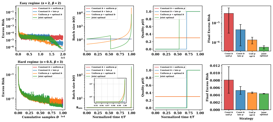
In the noise-limited regime, the training horizon is set to the joint optimal T ⋆ from Strategy 4
Constant b + uniform p: b(t) =D/T , p(t) =ρ . In the noise-limited regime, the training horizon is set to the joint optimal T ⋆ from Strategy 4. In the signal-limited regime, the constant batch is b=B min, which forces T=D/B min (the maximum feasible hori- zon)
-
[7]
Constant b + late p: same batch size and horizon as Strategy 1; quality is bang-bang 23 with p= 1 on the last ρT /η steps and p= 0 otherwise, satisfying the high-quality budget constraint
-
[8]
The training hori- zon T ⋆ is independently optimized by mini- mizing the FSL objective T −s +η R T 0 K(T− t)σ2 eff/b(t) dt over T using bounded scalar minimization
Uniform p + optimal b: p(t) =ρ throughout; batch size b(t) = max(C p K(T−t), B min) with the constant C determined by bisection so that R T 0 b(t) dt=D . The training hori- zon T ⋆ is independently optimized by mini- mizing the FSL objective T −s +η R T 0 K(T− t)σ2 eff/b(t) dt over T using bounded scalar minimization
-
[9]
Joint optimal: implements Theorem 4.3 di- rectly. In the noise-limited regime (Part I), the training horizon T ⋆ is optimized over T ; the batch schedule is b(t) =C p K(T ⋆ −t) on low-quality steps and b(t) =rC p K(T ⋆ −t) on high-quality steps, with quality placement chosen as late (one valid choice among the de- generate family). In the signal-limited r...
2025
discussion (0)
Sign in with ORCID, Apple, or X to comment. Anyone can read and Pith papers without signing in.