Dynamics of Stochastic Momentum with Sparse Updates in High Dimensions
Pith reviewed 2026-06-29 09:34 UTC · model grok-4.3
The pith
The phase structure of momentum with sparse updates in high dimensions is governed by the ratio of momentum retention and learning timescales.
A machine-rendered reading of the paper's core claim, the machinery that carries it, and where it could break.
Core claim
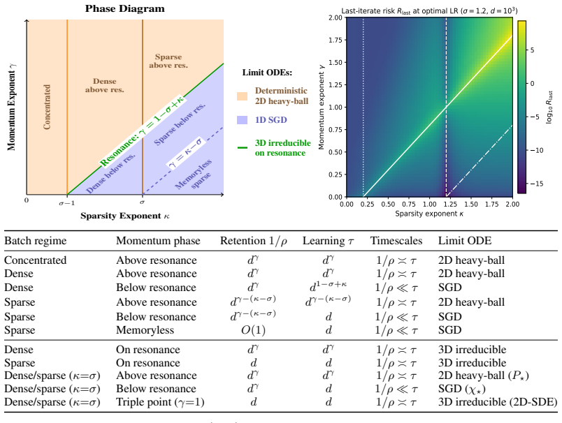
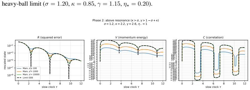
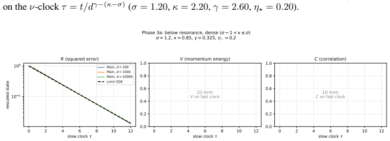
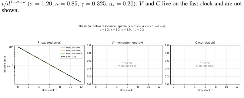
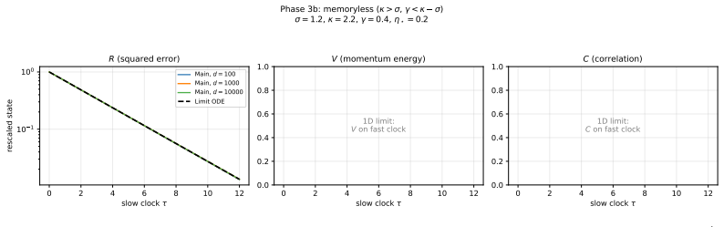
Both models admit exact closed-form second-moment dynamics whose high-dimensional limits are characterized across three scaling exponents. The phase structure is governed by the ratio of the momentum retention timescale to the learning timescale. When learning is much slower than retention the limit matches SGD, when faster the system is unstable, and when they coincide classical heavy-ball dynamics are recovered. Oscillatory dynamics occur at different momentum values for different token sparsity, creating a spectral conflict for global momentum across token frequencies.
What carries the argument
the ratio of the momentum retention timescale (how many active updates the buffer survives) to the learning timescale (how many active updates it takes to reduce the squared error)
If this is right
- When learning is much slower than retention, the high-dimensional limit matches SGD.
- When learning is faster than retention, the system is unstable.
- When the timescales coincide, classical heavy-ball dynamics are recovered.
- The oscillatory dynamics occur at different momentum values for different levels of token sparsity.
Where Pith is reading between the lines
- This implies that a single global momentum coefficient may be suboptimal in models where features or tokens have widely varying update frequencies, such as in language models.
- The timescale analysis could be used to predict optimal momentum decay rates from estimates of sparsity and error reduction rates in real datasets.
- Similar phase diagrams might exist for other momentum-like methods such as Nesterov acceleration or adaptive optimizers under sparse update conditions.
Load-bearing premise
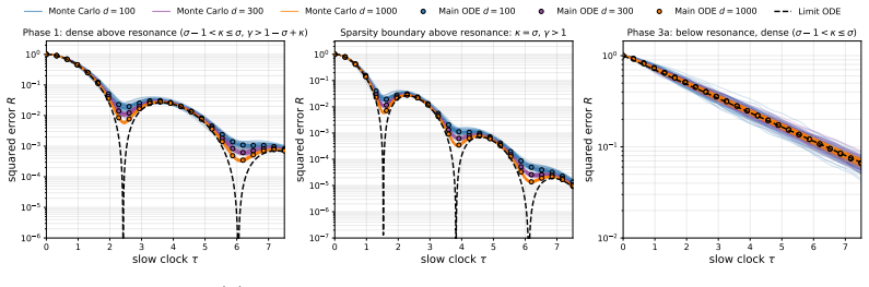
The two tractable models and the specific high-dimensional scaling regimes chosen for sparsity, batch size, and momentum decay are representative of the essential dynamics in practical high-dimensional settings with sparse updates.
What would settle it
A simulation of the least-squares model with sparse inputs that exhibits a phase transition at a momentum decay rate inconsistent with the predicted ratio of the two timescales would falsify the characterization of the high-dimensional limits.
Figures

read the original abstract
Existing theory of momentum assumes that gradients arrive at every parameter at a roughly constant rate, an assumption violated in practice by heavy-tailed data distributions and modern architectures. We theoretically analyze the dynamics of two tractable models of momentum under sparse updates: a least squares model with sparse inputs and a logistic regression model with a rare class. Both admit exact closed-form second-moment dynamics whose high-dimensional limits we characterize across three scaling exponents for sparsity, batch size, and momentum decay. The phase structure on both problems is governed by the ratio of two intrinsic timescales: a momentum retention timescale (how many active updates the buffer survives) and a learning timescale (how many active updates it takes to reduce the squared error). When learning is much slower than retention, the limit matches SGD; when learning is faster, the system is unstable; where the timescales coincide, we recover classical heavy-ball dynamics. The oscillatory dynamics occur at different momentum values for different token sparsity, creating a spectral conflict for global momentum across token frequencies.
Editorial analysis
A structured set of objections, weighed in public.
Referee Report
Summary. The paper analyzes dynamics of stochastic momentum under sparse updates using two tractable models (least squares with sparse inputs; logistic regression with rare class). It derives exact closed-form second-moment dynamics, takes high-dimensional limits across three scaling exponents (sparsity, batch size, momentum decay), and argues that the resulting phase structure is governed by the ratio of a momentum retention timescale to a learning timescale, recovering SGD-like, unstable, or classical heavy-ball regimes accordingly, plus a spectral conflict across token frequencies.
Significance. If the closed-form derivations and high-d limits hold, the work supplies a concrete mechanism (timescale ratio) explaining when momentum behaves like SGD versus heavy-ball under sparsity, a setting common in practice but outside standard momentum theory. The exact second-moment closures and falsifiable phase predictions constitute a clear strength.
major comments (2)
- [model sections and high-dimensional limit derivations] The central claim that the phase structure is governed by the retention-to-learning timescale ratio (and the associated SGD/unstable/heavy-ball limits) is derived entirely within the two chosen models. The manuscript does not supply evidence or additional analysis showing that coordinate-wise independent sparsity plus quadratic/logistic loss captures the essential dynamics when active coordinates are correlated or when feature interactions are nonlinear; this assumption is load-bearing for the generality of the timescale ratio as the governing quantity.
- [Abstract and high-d limit sections] Abstract and the high-d limit characterization: the exact closed-form second-moment dynamics are asserted to exist and to yield the stated phase diagram, yet the manuscript provides no explicit verification steps, error-bar handling, or cross-check against direct simulation of the finite-dimensional recursions that would confirm the limits are not artifacts of the scaling choices.
minor comments (1)
- [Abstract and introduction] Notation for the two intrinsic timescales is introduced in the abstract but would benefit from an explicit equation reference or definition box when first used in the main text.
Simulated Author's Rebuttal
We thank the referee for the constructive feedback. Below we address each major comment directly. We agree that the analysis is model-specific and will clarify scope; we also agree that numerical verification of the high-dimensional limits would strengthen the presentation and will incorporate it.
read point-by-point responses
-
Referee: [model sections and high-dimensional limit derivations] The central claim that the phase structure is governed by the retention-to-learning timescale ratio (and the associated SGD/unstable/heavy-ball limits) is derived entirely within the two chosen models. The manuscript does not supply evidence or additional analysis showing that coordinate-wise independent sparsity plus quadratic/logistic loss captures the essential dynamics when active coordinates are correlated or when feature interactions are nonlinear; this assumption is load-bearing for the generality of the timescale ratio as the governing quantity.
Authors: We agree that the derivations and resulting phase diagram are obtained strictly within the two tractable models (sparse-input least squares and rare-class logistic regression) that permit exact second-moment closures. These models assume coordinate-wise independent sparsity and do not incorporate correlations among active coordinates or nonlinear feature interactions. No additional analysis is provided for those regimes, as they generally destroy the exact solvability. The manuscript therefore establishes the timescale-ratio mechanism only for the stated models; we do not claim it governs arbitrary sparse-update settings. In revision we will add an explicit limitations paragraph in the discussion section stating the modeling assumptions and the consequent scope of the claimed phase structure. revision: yes
-
Referee: [Abstract and high-d limit sections] Abstract and the high-d limit characterization: the exact closed-form second-moment dynamics are asserted to exist and to yield the stated phase diagram, yet the manuscript provides no explicit verification steps, error-bar handling, or cross-check against direct simulation of the finite-dimensional recursions that would confirm the limits are not artifacts of the scaling choices.
Authors: The closed-form second-moment recursions are derived exactly in Sections 3 (least-squares model) and 4 (logistic model) by taking expectations over the sparse update process and solving the resulting linear system for the second-moment matrix. The high-dimensional limits are then obtained analytically in Section 5 by scaling the three exponents (sparsity, batch size, momentum decay) and extracting the dominant terms. While these steps are deterministic and exact under the model assumptions, we acknowledge that the manuscript contains no finite-dimensional numerical checks or error-bar comparisons. In the revision we will add a new subsection with direct simulations of the finite recursions for moderate dimensions, confirming convergence to the predicted phase boundaries as dimension grows. revision: yes
Circularity Check
No significant circularity; derivation self-contained from model equations
full rationale
The paper states that the two models admit exact closed-form second-moment dynamics derived directly from their defining equations, followed by high-dimensional limits taken across explicit scaling regimes for sparsity, batch size, and momentum decay. The phase structure is then characterized as a consequence of the resulting timescale ratio. No parameters are fitted to target outputs and then relabeled as predictions, no self-citations are invoked as load-bearing uniqueness theorems, and no ansatz or known result is smuggled in via prior work. The derivation chain therefore remains independent of the claimed conclusions.
Axiom & Free-Parameter Ledger
free parameters (1)
- three scaling exponents (sparsity, batch size, momentum decay)
axioms (2)
- domain assumption High-dimensional limits of the second-moment dynamics exist and admit exact characterization under the stated scalings
- domain assumption The sparse-input least-squares and rare-class logistic models capture the essential qualitative behavior of momentum under sparse updates in modern architectures
Reference graph
Works this paper leans on
-
[1]
Switch Transformers: Scaling to Trillion Parameter Models with Simple and Efficient Sparsity
URLhttps://arxiv.org/abs/2101.03961. Damien Ferbach, Katie Everett, Gauthier Gidel, Elliot Paquette, and Courtney Paquette. Dimension- adapted momentum outscales SGD, 2025. URLhttps://arxiv.org/abs/2505.16098. Damien Ferbach, Courtney Paquette, Gauthier Gidel, Katie Everett, and Elliot Paquette. Logarithmic- time schedules for scaling language models with...
work page internal anchor Pith review Pith/arXiv arXiv doi:10.1214/18-ejs1395 2025
-
[2]
URLhttps://arxiv.org/abs/1910.13962. Prateek Jain, Sham M. Kakade, Rahul Kidambi, Praneeth Netrapalli, and Aaron Sidford. Accelerating stochastic gradient descent for least squares regression. InProceedings of the 31st Conference on Learning Theory, volume 75 ofProceedings of Machine Learning Research, pages 545–604, 2018. URLhttps://proceedings.mlr.press...
-
[3]
Gated Attention for Large Language Models: Non-linearity, Sparsity, and Attention-Sink-Free
URLhttps://arxiv.org/abs/2505.06708. Othmane Sebbouh, Robert M. Gower, and Aaron Defazio. Almost sure convergence rates for stochastic gradient descent and stochastic heavy ball, 2021. URL https://arxiv.org/abs/ 2006.07867. Noam Shazeer. GLU variants improve transformer, 2020. URL https://arxiv.org/abs/2002. 05202. Noam Shazeer, Azalia Mirhoseini, Krzyszt...
work page internal anchor Pith review Pith/arXiv arXiv 2021
-
[4]
Understanding the Acceleration Phenomenon via High-Resolution Differential Equations
doi: 10.1007/s10107-021-01681-8. URLhttps://arxiv.org/abs/1810.08907. Yixin Song, Zeyu Mi, Haotong Xie, and Haibo Chen. PowerInfer: Fast large language model serving with a consumer-grade GPU. InProceedings of the ACM SIGOPS 30th Symposium on Operating Systems Principles, 2024. URLhttps://arxiv.org/abs/2312.12456. Weijie Su, Stephen Boyd, and Emmanuel J C...
work page internal anchor Pith review Pith/arXiv arXiv doi:10.1007/s10107-021-01681-8 2024
-
[5]
URLhttps://arxiv.org/abs/2307.15196. Shuche Wang, Fengzhuo Zhang, Jiaxiang Li, Cunxiao Du, Chao Du, Tianyu Pang, Zhuoran Yang, Mingyi Hong, and Vincent Y . F. Tan. Muon outperforms Adam in tail-end associative memory learning, 2025. URLhttps://arxiv.org/abs/2509.26030. Andre Wibisono, Ashia C. Wilson, and Michael I. Jordan. A variational perspective on ac...
-
[6]
URLhttps://arxiv.org/abs/1603.04245
doi: 10.1073/pnas.1614734113. URLhttps://arxiv.org/abs/1603.04245. Guangxuan Xiao, Yuandong Tian, Beidi Chen, Song Han, and Mike Lewis. Efficient streaming language models with attention sinks. InInternational Conference on Learning Representations,
-
[7]
Efficient Streaming Language Models with Attention Sinks
URLhttps://arxiv.org/abs/2309.17453. Jingyang Yuan, Huazuo Gao, Damai Dai, Junyu Luo, Liang Zhao, Zhengyan Zhang, Zhenda Xie, Y . X. Wei, Lean Wang, Zhiping Xiao, Yuqing Wang, Chong Ruan, Ming Zhang, Wenfeng Liang, and Wangding Zeng. Native sparse attention: Hardware-aligned and natively trainable sparse attention, 2025. URLhttps://arxiv.org/abs/2502.1108...
work page internal anchor Pith review Pith/arXiv arXiv 2025
-
[8]
hot” neurons fire on most inputs, while a heavy tail of “cold
construct a linear-regression instance on which standard stochastic heavy-ball and Nesterov schemes cannot outperform SGD for any choice of step size and momentum, and they propose an accelerated alternative that requires explicit oracle access. When acceleration over SGD is recovered, it is recovered by careful design. Jain et al. [2018] and Varre and Fl...
2018
-
[9]
κ= 0 corresponds to the dense limit; κ >0 captures sparse tokens or rare classes whose update / signal-arrival frequency decreases polynomially withd
Token / class sparsity (κ≥0 ):the gating probability p (or rare-class probability) scales as p≍d −κ. κ= 0 corresponds to the dense limit; κ >0 captures sparse tokens or rare classes whose update / signal-arrival frequency decreases polynomially withd
-
[10]
B(d) :=⌈d σ⌉; rounding does not affect polynomial-scale comparisons)
Mini-batch size (σ≥0 ):the batch size scales as B=B(d)≍d σ (e.g. B(d) :=⌈d σ⌉; rounding does not affect polynomial-scale comparisons). Typical values: σ= 0 (constant batch size, e.g. fine-tuning); σ= 1 (batch size proportional to dimension, e.g. large-scale pretraining)
-
[11]
Standard heavy-ball momentum corresponds to γ= 1 (i.e
Momentum decay ( γ≥0 ):the decay rate ε= 1−β scales as ε≍d −γ. Standard heavy-ball momentum corresponds to γ= 1 (i.e. β= 1−O(1/d) ); γ= 0 gives constant momentum independent ofd
-
[12]
squared drift
Learning rate (α):the learning rate scales as η≍d −α. The exponent α is determined by mean-square stability per region of the phase plane (cf. Appendix C.4 and the analogous LR analysis). For constant-level interior limits we sharpen the polynomial ansatz to p=p ∗d−κ(1 +o(1)), B=B ∗dσ(1 +o(1)), ε=ε ∗d−γ(1 +o(1)), η=η ∗d−α(1 +o(1)), (13) with fixed positiv...
-
[13]
The geometric waiting timeK∼Geometric(P batch)
-
[14]
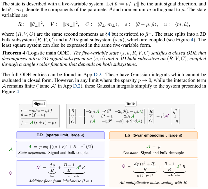
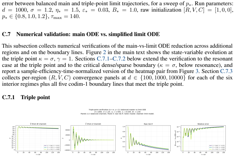
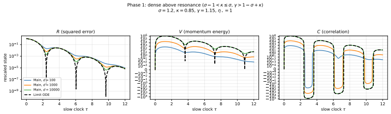
C.2.2 State Variables We derive closed ODEs for state variables R, V , and C by explicit expectation over the Gaussian model and the batch process
The content of the active batch (conditioned onN≥1). C.2.2 State Variables We derive closed ODEs for state variables R, V , and C by explicit expectation over the Gaussian model and the batch process. R(t) =E[∥Θ t −θ ∗∥2](total squared error) (47) V(t) =E[∥M t∥2](momentum second moment) (48) C(t) =E[⟨Θ t −θ ∗, Mt⟩](error-momentum correlation) (49) Remark5...
-
[15]
Diagonal terms (incoherent contribution).For isotropic Gaussian inputs x∼ N(0, I d) and fixede, the fourth-moment identity gives E ∥gi∥2 e =E ∥x∥2⟨x, e⟩2 = (d+ 2)∥e∥ 2.(56) Plugging into (55) yields 1 B2 X i∈S E ∥gi∥2 e = N B2 (d+ 2)∥e∥ 2.(57) Taking expectation overNconditioned on an active batch (N≥1) introducesB diag: E N B2 (d+ 2)∥e∥ 2 N≥1, e = (d+ 2)...
-
[16]
Cross terms (coherent contribution).Fori̸=j, usingg i =x ix⊤ i e, ⟨gi, gj⟩=e ⊤(xix⊤ i )(xjx⊤ j )e. Conditioned one, the inputsx i andx j are independent, hence E[⟨gi, gj⟩ |e] =e ⊤E[xix⊤ i ]E[x jx⊤ j ]e=e ⊤I I e=∥e∥ 2.(59) Summing over theN(N−1)ordered pairs and normalizing gives 1 B2 X i,j∈S i̸=j E[⟨gi, gj⟩ |e] = N(N−1) B2 ∥e∥2.(60) Taking expectation ove...
-
[17]
incoherent
Combined result and the B2 factor.Combining (58) and (61), we obtain the conditional second moment E ∥˜g∥2 N≥1, e = [(d+ 2)B diag +B cross]∥e∥ 2 =B 2 ∥e∥2,B 2 := (d+ 2)B diag +B cross. (62) Note thatB 2 scales the conditional second momentE[∥˜g∥2 |N≥1, e]and not a centered variance. Taking expectation over the randomness in the current error vector yields...
2026
-
[18]
c3 =o(ρ 3)), then exactly one root satisfies |λ|=o(ρ) , and this root is necessarily real
(1D scaling).If ˆc3 =o(1) (i.e. c3 =o(ρ 3)), then exactly one root satisfies |λ|=o(ρ) , and this root is necessarily real. Moreover, |λslow| ≍ c3 c2 . The remaining two roots satisfy|λ| ≍ρ. Proof.Letµ:=z/ρand write 0 =p(ρµ) =ρ 3 µ3 + ˆc1µ2 + ˆc2µ+ ˆc3 ,ˆc 1 := c1 ρ ,ˆc2 := c2 ρ2 ,ˆc3 := c3 ρ3 . By (180), ˆc1,ˆc2 are ≍1 . Cauchy’s root bound applied to the...
-
[19]
Hence c3 ≍ρ 3, and Lemma 14 implies that all three eigenvalues satisfy |λ| ≍ρ , i.e
3D regimes (correlation-limited).In the 3D regimes, the binding ceiling is correlation- limited, so ηB1 ≍ρ (at polynomial resolution). Hence c3 ≍ρ 3, and Lemma 14 implies that all three eigenvalues satisfy |λ| ≍ρ , i.e. all three modes relax on the retention-controlled timescaleτ≍ρ −1
-
[20]
Hence c3 =o(ρ 3), and Lemma 14 implies there is a unique eigenvalue λslow with |λslow| ≍ c3 c2 ≍ηB 1 ≪ρ, while the other two eigenvalues satisfy |λ| ≍ρ
1D regimes (noise-limited or memoryless).In the 1D regimes, ηB1 ≪ρ at polynomial resolution. Hence c3 =o(ρ 3), and Lemma 14 implies there is a unique eigenvalue λslow with |λslow| ≍ c3 c2 ≍ηB 1 ≪ρ, while the other two eigenvalues satisfy |λ| ≍ρ . Equivalently, there is a strict separation between one slow mode and a fast cluster: τfast ≲ρ −1 ≪τ slow ≍(ηB ...
-
[21]
Draw Y∼Bernoulli(p) , with Y= 2 (the rare class) having probability p and Y= 1 (the common class) having probability1−p
-
[22]
DrawZ∼ N(0, I d)independently ofY
-
[23]
The common class is unstructured Gaussian noise; all signal about µ is carried by the rare class
SetX:=µ+ZifY= 2, andX:=ZifY= 1. The common class is unstructured Gaussian noise; all signal about µ is carried by the rare class. We write˜y:=1{y= 2} ∈ {0,1}for the binary label. D.1.2 Logistic model and gradient We fit a binary logistic model with parameters(θ, b)∈R d ×R, Pθ,b(Y= 2|X=x) =σ ⟨θ, x⟩+b , σ(z) := ez 1 +e z ,(189) with logistic loss ℓ(θ, b;x, ...
-
[24]
LR: 2D in (s, R⊥)
Slow-manifold dimension.LS: 1D in R. LR: 2D in (s, R⊥). The signal damping rate ηpα matches the bulk slow rate and the signal cannot be adiabatically eliminated alongside the momentum
-
[25]
homogeneous bulk.LS: ˙R=−c effR with R∗ = 0
Affine vs. homogeneous bulk.LS: ˙R=−c effR with R∗ = 0. LR: ˙R⊥ =−2η ∗p∗αR⊥ + η∗p∗ηeff with strict positive floorR ∗ ⊥ >0
-
[26]
No LS analog
Exponential coupling through α.The factor α=e ((s+r)2+R⊥−r2)/2 couples s and R⊥ through a state-dependent effective rate. No LS analog
-
[27]
s∗ ̸= 0 in LR (eq
Signal bias. s∗ ̸= 0 in LR (eq. (248)); LS has no separate signal slow variable below resonance
-
[28]
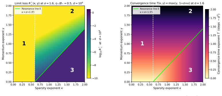
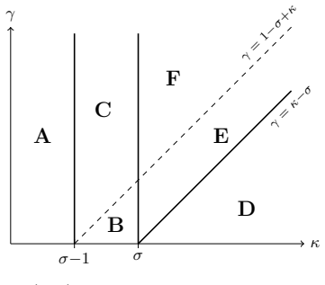
Stability mechanism.LS sparse-below-resonance has a stability threshold ηeff <2 from ceff >0 . LR’s bulk damping −2ηpα <0 is unconditionally contractive; the ηeff =O(1) constraint here comes fromfloor control( R∗ ⊥ =O(1) keeps α=O(1) and the tame-α approximation valid), not from stability. D.5.5 Boundary E: resonance lineγ= 1−σ+κ Region.The 1D locus where...
-
[29]
The LS batching regimes collapse into a partition by noise character (κ≶σ−1 ) and resonance (γ≶1−σ+κ )
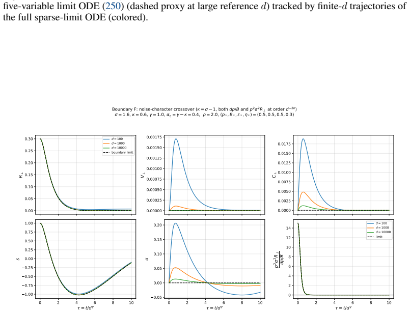
The dense/sparse boundary κ=σ disappears.Every step is active in logistic ( Pbatch ≡ 1), so the LS sparse-batching cutoff at κ=σ has no logistic counterpart. The LS batching regimes collapse into a partition by noise character (κ≶σ−1 ) and resonance (γ≶1−σ+κ )
-
[30]
It is intrinsically nonlinear: LS has only multiplicative bulk noise, no analog of the additivedp/Bchannel
A new noise-character boundary κ=σ−1 appears(Boundary F). It is intrinsically nonlinear: LS has only multiplicative bulk noise, no analog of the additivedp/Bchannel
-
[31]
The below-resonance noise-floor regime is genuinely novel.The coupled 2D slow manifold (s, R⊥) with affine noise-floor forcing and nonlinearα-coupling has no LS analog. The signal cannot be adiabatically eliminated because its damping rate ηpα is at the same slow timescale as the bulk; the equilibrium signal is biased away from the population optimum by t...
-
[32]
Above resonance, the additive noise floor exists at every finited but vanishes in the limit; the leading dynamics coincide with the concentrated above-resonance regime
The above-resonance noise-floor regime carries a vanishing floorR∗ ⊥(d)≍d 1−σ+κ−2γ. Above resonance, the additive noise floor exists at every finited but vanishes in the limit; the leading dynamics coincide with the concentrated above-resonance regime. This is the bias/speed trade-off of Section 6
-
[33]
Logistic-specific signal-direction curvature 1 +r 2.The factor enters the heavy-ball curvature in the above-resonance regimes and Boundary E, and the linearized Jacobian in the below-resonance noise-floor regime; no LS analog (LS curvature is1)
-
[34]
decoupled heavy-ball
Bias against perfect alignment in noise-floor regimes.In the below-resonance noise- floor regime, the floor R∗ ⊥ >0 forces α∗ >1 , shifting the equilibrium signal to s∗ = r(1/α∗ −1)<0. LS has no separate signal slow variable. Triple-point structure.The codim-2 stratum κ=σ−1 , γ= 0 (F∩E ) is the unique point where (i) both noise channels survive at ≍1 and ...
discussion (0)
Sign in with ORCID, Apple, or X to comment. Anyone can read and Pith papers without signing in.