BV pushforward as a quasi-isomorphism
Pith reviewed 2026-06-29 00:10 UTC · model grok-4.3
The pith
The BV pushforward map is a quasi-isomorphism of BV complexes when fields are split into infrared and ultraviolet subspaces.
A machine-rendered reading of the paper's core claim, the machinery that carries it, and where it could break.
Core claim
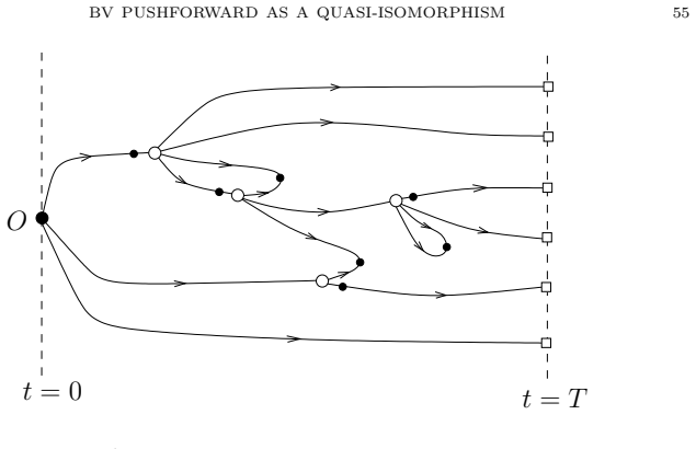
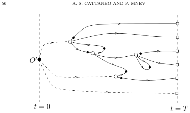
In a BV theory on fields split into infrared and ultraviolet parts, the BV pushforward P_* is part of a strong deformation retraction and therefore a quasi-isomorphism of the BV complexes, with the quasi-inverse i_int realized as a path integral in the topological quantum mechanics perspective.
What carries the argument
Strong deformation retraction constructed via the homological perturbation lemma, with P_* as one component and i_int as the quasi-inverse.
If this is right
- The induced map on BV cohomology is an isomorphism, so physical observables are preserved.
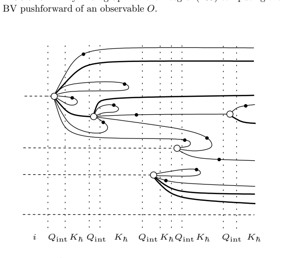
- An explicit formula for lifting effective observables to the full theory is obtained.
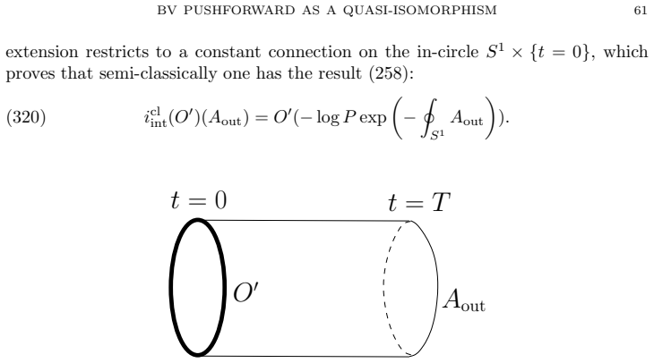
- The classical limit of the lifting map can be studied using the AKSZ realization.
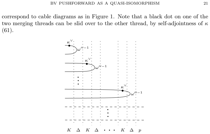
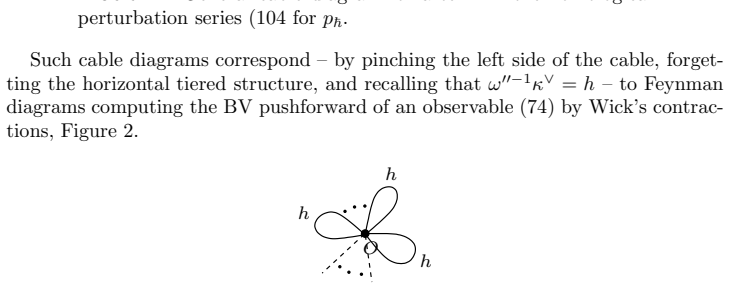
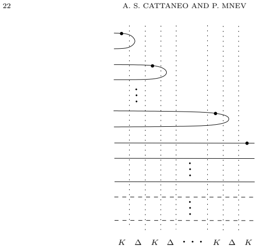
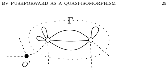
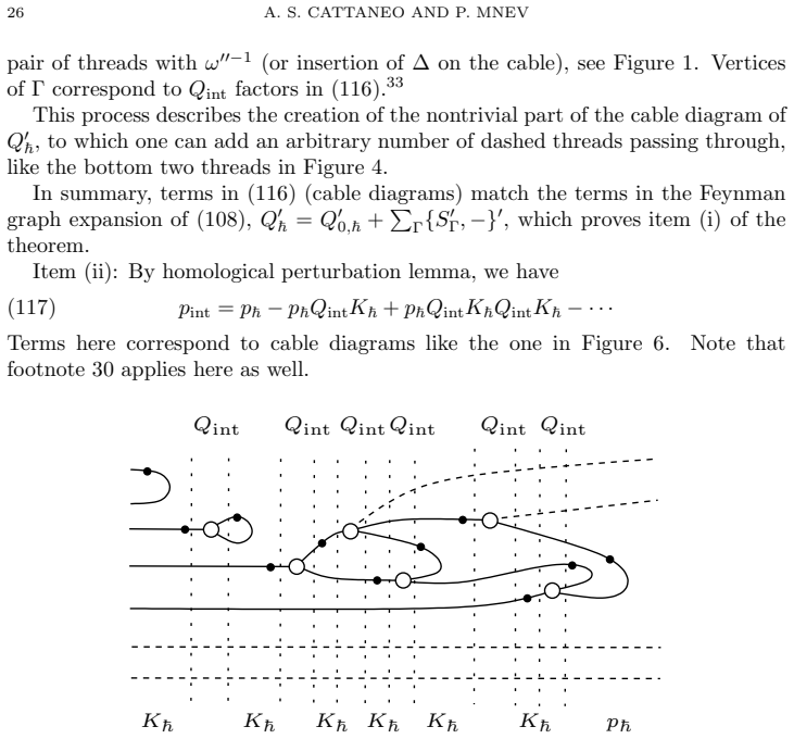
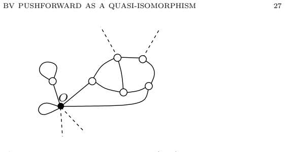
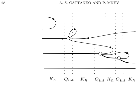
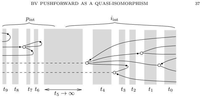
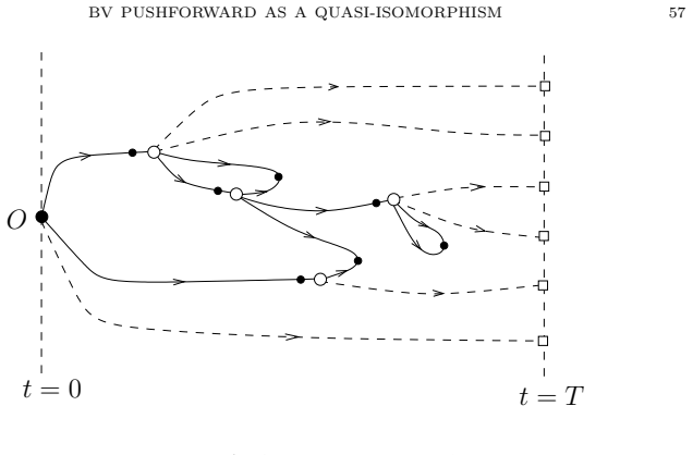
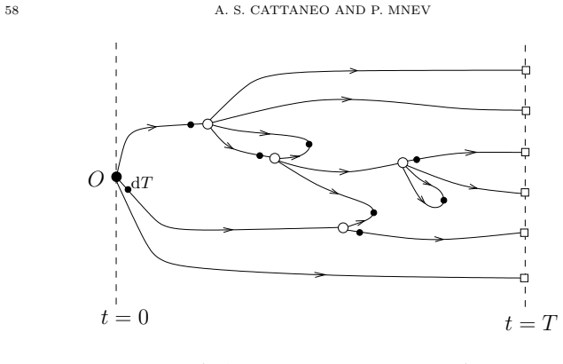
- Feynman diagrams for the pushforward correspond to cable diagrams from perturbation theory.
Where Pith is reading between the lines
- This equivalence suggests that computations in the effective theory capture the same cohomological information as the full theory.
- The path integral form of i_int may allow numerical or approximate evaluations in specific models.
- Similar retraction constructions could apply to other field splittings or gauge theories.
Load-bearing premise
The space of fields admits a splitting into infrared and ultraviolet subspaces on which a BV theory is defined.
What would settle it
Construct a concrete BV theory with an infrared-ultraviolet field split where the pushforward map fails to induce an isomorphism on the cohomology of the BV operator.
Figures
read the original abstract
Given a BV theory on a space of fields split into two subspaces ("infrared" and "ultraviolet"), one has the BV pushforward map $P_*$, sending observables to observables of the effective theory on the infrared space. This note proves that $P_*$ is a quasi-isomorphism of BV complexes, by realizing it as a part of a strong deformation retraction constructed using the homological perturbation lemma. Two proofs are given: (i) comparing Feynman diagrams for $P_*$ with "cable diagrams" arising from homological perturbation theory and (ii) using topological quantum mechanics. This construction gives a formula for the quasi-inverse $i_\mathrm{int}$ of $P_*$ - the map lifting observables of the effective theory to the full theory. The topological quantum mechanics perspective - and its realization as an AKSZ theory - allows one to write $i_\mathrm{int}$ as a path integral (realizing cable diagrams for $i_\mathrm{int}$ as Feynman diagrams) and to study its classical limit.
Editorial analysis
A structured set of objections, weighed in public.
Referee Report
Summary. Given a BV theory on a space of fields split into infrared and ultraviolet subspaces, the manuscript proves that the BV pushforward map P_* is a quasi-isomorphism of BV complexes. It realizes P_* as part of a strong deformation retraction constructed via the homological perturbation lemma. Two proofs are supplied: one equating the Feynman diagrams of P_* with cable diagrams from HPL, and the other realizing the construction inside an AKSZ model via topological quantum mechanics. The work also supplies an explicit formula for the quasi-inverse i_int, which admits a path-integral representation whose classical limit can be studied.
Significance. If the result holds, it supplies a rigorous justification, via standard homological algebra, for the quasi-isomorphism property of the BV pushforward that underlies effective BV theories. The two independent proofs, the explicit quasi-inverse, and the AKSZ/topological-QM realization (which converts cable diagrams into Feynman diagrams) are concrete strengths that increase the reliability of the claim.
minor comments (1)
- [Abstract] The abstract introduces 'cable diagrams' without a one-sentence gloss or forward reference; a brief parenthetical would improve immediate readability for readers outside the immediate subfield.
Simulated Author's Rebuttal
We thank the referee for their positive summary, recognition of the significance of the result, and recommendation of minor revision. No specific major comments were listed in the report.
Circularity Check
No significant circularity
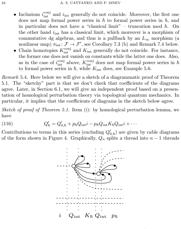
full rationale
The derivation assumes the field-space splitting into IR/UV subspaces as an explicit setup hypothesis and then invokes the standard homological perturbation lemma to build a strong deformation retraction containing P_*. The two proofs—one equating Feynman diagrams of P_* with HPL cable diagrams and the other realizing the construction inside an AKSZ model via topological quantum mechanics—supply an explicit quasi-inverse i_int without reducing any claim to a self-definition, a fitted parameter renamed as a prediction, or a load-bearing self-citation chain. All steps rely on external, independently verifiable mathematical machinery rather than internal re-labeling of inputs.
Axiom & Free-Parameter Ledger
axioms (1)
- standard math The homological perturbation lemma applies to the BV complexes arising from the infrared-ultraviolet splitting.
Reference graph
Works this paper leans on
-
[1]
The geometry of the master equation and topological quantum field theory
M. Alexandrov, M. Kontsevich, A. Schwarz, O. Zaboronsky . “The geometry of the master equation and topological quantum field theory.” Internatio nal Journal of Modern Physics A 12, no. 07 (1997): 1405–1429
1997
-
[2]
How to discretize the different ial forms on the interval
R. Bandiera, F. Schaetz, “How to discretize the different ial forms on the interval.” Higher Structures 1 (2017): 56–86
2017
-
[3]
Burghart, J
F. Burghart, J. Steinebrunner, Unpublished undergradu ate student intern project directed by P. Mnev, Max Planck Insitute for Mathematics, Bonn, 2015
2015
-
[4]
Minimal models in algebra, combinatorics and topology,
A. Berglund, “Minimal models in algebra, combinatorics and topology,” PhD thesis, Stock- holm University 2008
2008
-
[5]
Towards equivar iant Yang–Mills theory
F. Bonechi, A. S. Cattaneo, M. Zabzine, “Towards equivar iant Yang–Mills theory.” Journal of Geometry and Physics 189 (2023): 104836
2023
-
[6]
Surface Observables, 2-Knot Invariant s, and Nonabelian Electric Fluxes
A. S. Cattaneo, “Surface Observables, 2-Knot Invariant s, and Nonabelian Electric Fluxes.” arXiv preprint arXiv:2511.13623 (2025)
-
[7]
Perturbative q uantum gauge theories on manifolds with boundary
A. S. Cattaneo, P. Mnev, N. Reshetikhin. “Perturbative q uantum gauge theories on manifolds with boundary.” Communications in Mathematical Physics 357.2 (2018): 631–730
2018
-
[8]
A cellular topo logical field theory
A. S. Cattaneo, P. Mnev, N. Reshetikhin. “A cellular topo logical field theory.” Communica- tions in Mathematical Physics 374.2 (2020): 1229–1320
2020
-
[9]
Higher-Dimensional BF Theories in the Batalin–Vilkovisky For- malism: The BV Action and Generalized Wilson Loops
A. S. Cattaneo, C. A. Rossi. “Higher-Dimensional BF Theories in the Batalin–Vilkovisky For- malism: The BV Action and Generalized Wilson Loops.” Commun ications in Mathematical physics 221.3 (2001): 591–657
2001
-
[10]
Factorization Algebras in Q uantum Field Theory
K. Costello, O. Gwilliam. “Factorization Algebras in Q uantum Field Theory.” Vol. 2. Cam- bridge University Press, 2021
2021
-
[11]
On the perturbation lemma, and deformations
M. Crainic. “On the perturbation lemma, and deformatio ns.” 2004. arXiv: math/0403266v1 [math.AT]
work page internal anchor Pith review Pith/arXiv arXiv 2004
-
[12]
Lie theory for nilpotent L∞ -algebras
E. Getzler, “Lie theory for nilpotent L∞ -algebras.” Annals of mathematics (2009): 271–301
2009
-
[13]
Cyclic L∞ algebras and shifted symplectic forms,
E. Getzler, “Cyclic L∞ algebras and shifted symplectic forms,” talk at the confere nce “Fifty years of BRST,” Munich, March 24, 2026
2026
-
[14]
Perturbation theory in differential homological algebra I
V. K. Gugenheim and L. A. Lambe. “Perturbation theory in differential homological algebra I.” In: Illinois Journal of Mathematics 33.4 (1989), pp. 566 –582. 62 A. S. CATTANEO AND P. MNEV
1989
-
[15]
Geometry of localized effective the ories, exact semi-classical approx- imation and the algebraic index
Z. Gui, S. Li, K. Xu. “Geometry of localized effective the ories, exact semi-classical approx- imation and the algebraic index.” Communications in Mathem atical Physics 382.1 (2021): 441–483
2021
-
[16]
Elliptic trace map on chiral algebras
Z. Gui, S. Li. “Elliptic trace map on chiral algebras.” a rXiv preprint arXiv:2112.14572 (2021)
-
[17]
Factorization algebras and free field the ories
O. Gwilliam, “Factorization algebras and free field the ories.” Northwestern University, 2012
2012
-
[18]
How to derive Feynman diagrams for finite-dimensional integrals directly from the BV formalism,
O. Gwilliam, T. Johnson-Freyd. “How to derive Feynman d iagrams for finite-dimensional integrals directly from the BV formalism.” arXiv preprint a rXiv:1202.1554 (2012)
-
[19]
Formal solution of the mas ter equa- tion via HPT and defor- mation theory
J. Huebschmann, J. Stasheff. “Formal solution of the mas ter equa- tion via HPT and defor- mation theory.” Forum Math. 14 (2002): 847–868
2002
-
[20]
Homological perturbation theory f or nonperturbative integrals
T. Johnson-Freyd, “Homological perturbation theory f or nonperturbative integrals.” Letters in Mathematical Physics 105.11 (2015): 1605-1632
2015
-
[21]
Semidensities on odd symplectic s upermanifolds
H. M. Khudaverdian, “Semidensities on odd symplectic s upermanifolds.” Communications in mathematical physics 247.2 (2004): 353–390
2004
-
[22]
Quantum field theory as effective BV theory from Chern–Simons
D. Krotov, A. Losev. “Quantum field theory as effective BV theory from Chern–Simons.” Nuclear physics B 806, no. 3 (2009): 529–566
2009
-
[23]
Vertex algebras and quantum master equation
S. Li. “Vertex algebras and quantum master equation.” J ournal of Differential Geometry 123.3 (2023): 461–521
2023
-
[24]
BV formalism and quantum homotopical struct ures
A. Losev, “BV formalism and quantum homotopical struct ures.” Lectures at GAP3, Perugia, 2005
2005
-
[25]
TQFT, homological algebra and elements of K. Saito’s theory of primitive form: an attempt of mathematical text written by mathematical phy sicist
A. Losev, “TQFT, homological algebra and elements of K. Saito’s theory of primitive form: an attempt of mathematical text written by mathematical phy sicist.” In Primitive Forms and Related Subjects—Kavli IPMU 2014 , vol. 83, pp. 269–294. Mathematical Society of Japan, 2019
2014
-
[26]
Notes on simplicial BF theory
P. Mnev, “Notes on simplicial BF theory.” Moscow Mathematical Journal 9.2 (2009): 371– 410
2009
-
[27]
P. Mnev, “Discrete BF theory.” arXiv preprint arXiv:0809.1160 (2008)
work page internal anchor Pith review Pith/arXiv arXiv 2008
-
[28]
Pert urbative quantum field theory and homotopy algebras
C. Saemann, B. Jurco, H. Kim, T. Macrelli, M. W olf. “Pert urbative quantum field theory and homotopy algebras.” In Proceedings of Corfu Summer Institute 2019 “School and Work shops on Elementary Particle Physics and Gravity”—PoS (CORFU201 9). Proceedings Of Science, 2020
2019
-
[29]
Symmetry factors of Feynm an diagrams and the homological perturbation lemma
C. Saemann, E. Sfinarolakis. “Symmetry factors of Feynm an diagrams and the homological perturbation lemma.” Journal of High Energy Physics 2020.1 2 (2020): 88
2020
-
[30]
Geometry of Batalin–Vilkovisky quantiza tion
A. Schwarz. “Geometry of Batalin–Vilkovisky quantiza tion.” Communications in Mathemat- ical Physics 155.2 (1993): 249–260
1993
-
[31]
On the origin of the BV operator on odd symplectic su permanifolds
P. ˇSevera. “On the origin of the BV operator on odd symplectic su permanifolds.” Letters in Mathematical Physics 78.1 (2006): 55–59. Institut f ¨ur Mathematik, Universit ¨at Z ¨urich, Winterthurerstrasse 190, CH-8057 Z¨urich, Switzerland Email address : cattaneo@math.uzh.ch University of Notre Dame, Notre Dame, IN 46556, USA Institut f ¨ur Mathematik, Un...
2006
discussion (0)
Sign in with ORCID, Apple, or X to comment. Anyone can read and Pith papers without signing in.