What Makes a Strong Model? A Unified Spectral Analysis of Knowledge Transfer over High-dimensional Linear Regression
Pith reviewed 2026-06-28 17:16 UTC · model grok-4.3
The pith
Knowledge transfer efficacy arises from the interplay of implicit regularization and heterogeneous spectral learning speeds in SGD dynamics.
A machine-rendered reading of the paper's core claim, the machinery that carries it, and where it could break.
Core claim
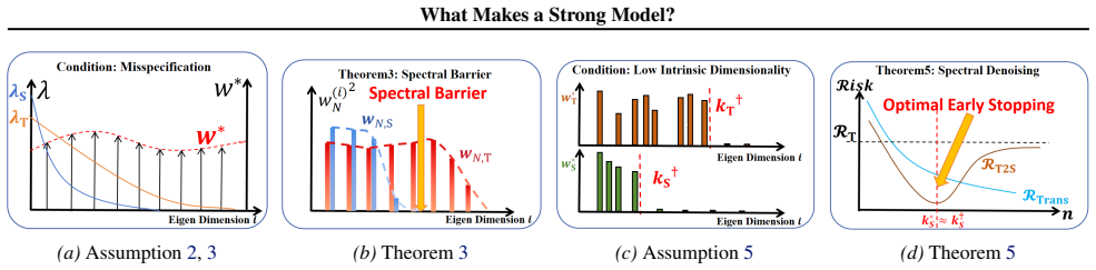
The efficacy of teacher-student knowledge transfer is governed by the interplay between implicit regularization and heterogeneous spectral learning speeds over the spectrum, which produces spectral horizon expansion in knowledge distillation and spectral denoising in weak-to-strong generalization.
What carries the argument
The spectral analysis of SGD dynamics, which tracks learning speeds and regularization effects separately across frequency components of the data covariance.
If this is right
- Knowledge distillation succeeds when the teacher provides access to high-frequency modes that the student could not reach within its training horizon.
- Weak-to-strong generalization occurs when the stronger model filters optimization noise that the weaker model would otherwise amplify.
- Transfer performance can be diagnosed by comparing the eigenvalue decay of the data covariance against the regularization strength induced by SGD.
- Heterogeneous learning speeds across the spectrum determine whether transfer improves or degrades final generalization.
Where Pith is reading between the lines
- The same spectral lens could be applied to compare different optimizers by measuring how each shapes the effective regularization profile over frequencies.
- If the unification holds, one could design data-dependent curricula that deliberately align student learning speeds with teacher-provided signals.
- The analysis suggests testing whether spectral denoising persists when the student and teacher use mismatched architectures but share the same data spectrum.
Load-bearing premise
The high-dimensional linear regression setting with SGD dynamics captures the essential mechanisms of knowledge transfer that apply more broadly to neural network training regimes.
What would settle it
A controlled experiment in which the spectrum of the covariance matrix is altered so that all frequency components learn at identical speeds, after which knowledge transfer should lose its predicted advantage over direct training.
Figures
read the original abstract
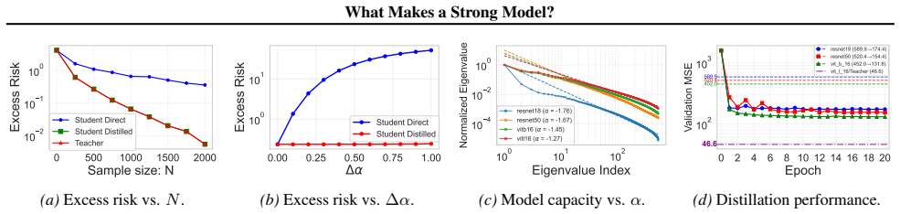
Teacher-Student Knowledge Transfer (KT) is ubiquitous in modern machine learning, ranging from classical model compression via Knowledge Distillation (KD) to the emergent phenomenon of Weak-to-Strong (W2S) generalization. While existing studies offer isolated insights, a unified theoretical framework explaining the efficacy of KT across these disparate regimes remains lacking. In this work, we establish a unified spectral analysis of SGD dynamics in high-dimensional linear regression, elucidating the efficiency of KT across seemingly disparate regimes. We characterize KT efficiency through two distinct mechanisms: \emph{Spectral Horizon Expansion} in KD, which enables the capture of statistically inaccessible high-frequency signals, and \emph{Spectral Denoising} in W2S, where the student acts as a filter for optimization noise. Our framework unifies these phenomena, revealing that the efficacy of transfer is governed by the interplay between implicit regularization and heterogeneous spectral learning speeds over the spectrum.
Editorial analysis
A structured set of objections, weighed in public.
Referee Report
Summary. The paper claims to establish a unified spectral analysis of SGD dynamics in high-dimensional linear regression that explains knowledge transfer (KT) efficacy across knowledge distillation (KD) and weak-to-strong (W2S) regimes. It characterizes KT efficiency via two mechanisms—Spectral Horizon Expansion in KD (capturing high-frequency signals) and Spectral Denoising in W2S (filtering optimization noise)—governed by the interplay of implicit regularization and heterogeneous spectral learning speeds over the spectrum.
Significance. If the derivations hold, the work provides a coherent linear-model framework that unifies isolated KT observations through spectral properties of SGD, offering explicit mechanisms (horizon expansion, denoising) tied to regularization and learning speeds. This is a strength for the linear setting, though the manuscript does not ship machine-checked proofs or reproducible code.
major comments (2)
- [§1] The central unification claim rests on the premise that high-dimensional linear regression with SGD captures the essential mechanisms of KT that apply to neural networks (§1, abstract). No derivation or experiment demonstrates that Spectral Horizon Expansion or Spectral Denoising survive the introduction of nonlinear activations, depth, or attention, which alter both the spectrum and effective regularization; this is load-bearing for the claim that the framework explains efficacy 'across these disparate regimes.'
- [model section / main theorems] The definitions of Spectral Horizon Expansion and Spectral Denoising appear to be introduced specifically for the linear case without a general mapping to nonlinear KT; if these reduce to properties of the covariance spectrum under linear SGD, the unification may be tautological to the model choice rather than explanatory for broader KT (model section and main theorems).
minor comments (2)
- Notation for the spectrum and learning speeds should be defined with explicit equations early in the paper to improve readability.
- [abstract] The abstract states the framework 'unifies these phenomena' but does not preview the precise conditions under which the two mechanisms dominate; a short statement of the regime boundaries would help.
Simulated Author's Rebuttal
We thank the referee for the constructive comments. Our work derives exact mechanisms for knowledge transfer in the high-dimensional linear regression setting under SGD, unifying KD and W2S through spectral properties. We address the major comments below, clarifying scope without overstating generality.
read point-by-point responses
-
Referee: [§1] The central unification claim rests on the premise that high-dimensional linear regression with SGD captures the essential mechanisms of KT that apply to neural networks (§1, abstract). No derivation or experiment demonstrates that Spectral Horizon Expansion or Spectral Denoising survive the introduction of nonlinear activations, depth, or attention, which alter both the spectrum and effective regularization; this is load-bearing for the claim that the framework explains efficacy 'across these disparate regimes.'
Authors: We agree that the manuscript is confined to the linear setting and provides neither derivations nor experiments for nonlinear activations, depth, or attention. The abstract and §1 explicitly frame the contribution as a unified spectral analysis of SGD dynamics in high-dimensional linear regression to elucidate KT efficiency across KD and W2S regimes. The unification claim concerns these two regimes within the linear model, not direct applicability to neural networks. We will revise the introduction and conclusion to state the scope more explicitly and add a limitations paragraph discussing why nonlinear extensions require separate analysis. This is a partial revision. revision: partial
-
Referee: [model section / main theorems] The definitions of Spectral Horizon Expansion and Spectral Denoising appear to be introduced specifically for the linear case without a general mapping to nonlinear KT; if these reduce to properties of the covariance spectrum under linear SGD, the unification may be tautological to the model choice rather than explanatory for broader KT (model section and main theorems).
Authors: The definitions arise from the closed-form SGD dynamics on the covariance spectrum, incorporating implicit regularization and mode-dependent learning speeds; they are not presupposed but derived as consequences that distinguish KD (horizon expansion via teacher guidance) from W2S (denoising via student filtering). This yields testable predictions on transfer efficacy that match simulations, providing explanatory power beyond merely restating the spectrum. The linear model is chosen precisely because it permits such exact characterization; we do not claim a general mapping to nonlinear KT. No revision is required on this point. revision: no
Circularity Check
No circularity in provided derivation description
full rationale
The abstract and reader's summary describe a spectral analysis of SGD in high-dimensional linear regression that characterizes KT via Spectral Horizon Expansion and Spectral Denoising, governed by implicit regularization and heterogeneous learning speeds. No equations, fitted parameters renamed as predictions, self-definitional constructs, or load-bearing self-citations are quoted or visible. The framework is presented as an independent modeling choice whose central unification claim does not reduce to its inputs by construction, satisfying the criteria for a self-contained derivation with no detected circular steps.
Axiom & Free-Parameter Ledger
Reference graph
Works this paper leans on
-
[1]
Scaling and renormalization in high-dimensional regression
URL https://api.semanticscholar. org/CorpusID:258509089. Allen-Zhu, Z. and Li, Y . Towards understanding ensemble, knowledge distillation and self-distillation in deep learn- ing, 2023. URL https://arxiv.org/abs/2012. 09816. Atanasov, A., Zavatone-Veth, J. A., and Pehlevan, C. Scaling and renormalization in high-dimensional regression.ArXiv, abs/2405.0059...
work page internal anchor Pith review Pith/arXiv arXiv doi:10.1073/pnas.1907378117 2023
-
[2]
doi: 10.1038/s41586-025-09422-z
URL https://api.semanticscholar. org/CorpusID:266312608. Caron, M., Touvron, H., Misra, I., J ´egou, H., Mairal, J., Bojanowski, P., and Joulin, A. Emerging properties in self-supervised vision transformers. InProceedings of the IEEE/CVF international conference on computer vision, pp. 9650–9660, 2021. Charikar, M., Pabbaraju, C., and Shiragur, K. Quantif...
-
[3]
URL https://api.semanticscholar. org/CorpusID:273185855. Wu, J., Zou, D., Braverman, V ., Gu, Q., and Kakade, S. Last iterate risk bounds of SGD with decaying stepsize for overparameterized linear regression. InInternational Conference on Machine Learning, 2022. Zhang, H., Liu, Y ., Chen, Q., and Fang, C. The optimality of (accelerated) sgd for high-dimen...
-
[4]
We take the trace of the RHS of Eq
Derivation of Excess Risk.The expected excess risk is given by E[E(w N)] = 1 2tr(ΣE[η N ⊗η N]). We take the trace of the RHS of Eq. (1) against 1 2Σ. Variance Part: 1 2tr Σ·(Σ ≤k∗ )−1 = 1 2 k∗ X i=1 λi · 1 λi = k∗ 2 ,(96) 1 2tr Σ·Σ >k∗ = 1 2 dX i=k∗+1 λ2 i .(97) Applying the pre-factor32(. . .), the variance contribution becomes16(ψ∥η 0∥2 Σ +σ 2 eff)( k∗ ...
-
[5]
If the target functionw ∗ is not fully realizable within the feature space (i.e., w∗ has a component in the null space of Σ), an irreducible approximation error exists
Total Risk.The total riskR(w N)is defined over the entire input space. If the target functionw ∗ is not fully realizable within the feature space (i.e., w∗ has a component in the null space of Σ), an irreducible approximation error exists. By the Pythagorean theorem in the Hilbert space, this error is orthogonal to the estimation error, yielding the addit...
-
[6]
Bias Component:From Lemma 13, we established the lower bound for the bias energy in the tail subspace: tr(ΣBN)≥ NY i=1 (I−γ iΣ)η0 2 Σ>k∗ ≥ 1 100 ∥η0∥2 Σ>k∗ .(109) Multiplying by the factor 1 2 from the risk definition yields the first term 1 200 ∥η0∥2 Σ>k∗
-
[7]
Variance Component:From Lemma 14, the variance matrix satisfies CN ⪰ σ2 eff 4 (γ0I≤k∗ +Kγ 2 0Σ>k∗ ). Applying the trace operator 1 2tr(Σ·): For theTail part(k > k ∗): 1 2tr Σ· σ2 eff 4 Kγ 2 0Σ>k∗ = σ2 eff 8 Kγ 2 0 dX i=k∗+1 λ2 i .(110) For theHead part(k≤k ∗): 1 2tr Σ· σ2 eff 4 γ0I≤k∗ = σ2 eff 8 k∗ X i=1 γ0λi.(111) We now connect the termP γ0λi to k∗/K. B...
-
[8]
Replace the sample sizeNwith the student’s training stepsn
-
[9]
Replace the generic covarianceΣwithΣ S and its eigenvaluesλ k,S
-
[10]
Replace the initial error norms∥η 0∥2 (·) with the teacher’s norms∥wN,T∥2 (·)
-
[11]
Replace the noise varianceσ 2 eff with the transfer residualˆσ2
-
[12]
Then we shall have the desired upper bound
Replace the stepsize intervalKwithK ′ =n/log 2 n. Then we shall have the desired upper bound. B.2. Proof of Geometric Consistency Condition (Lemma 2) We derive the consistency condition by explicitly comparing the optimal parameters obtained via Direct Learning versus Knowledge Transfer using the Moore-Penrose pseudoinverse properties. Proof. Let the grou...
-
[13]
The minimal-norm solution tomin w ∥M⊤ S w−w ∗∥2 is: w∗ S = (M⊤ S )+w∗.(130) Knowledge Transfer:The teacher first learns the ground truth, yielding w∗ T = (M⊤ T)+w∗
Optimal Parameters Derivation Direct Learning:The student directly approximatesw ∗. The minimal-norm solution tomin w ∥M⊤ S w−w ∗∥2 is: w∗ S = (M⊤ S )+w∗.(130) Knowledge Transfer:The teacher first learns the ground truth, yielding w∗ T = (M⊤ T)+w∗. The student then mimics the teacher’s effective parameterwT,eff =M ⊤ Tw∗ T =Π Tw∗. The student’s optimal sol...
-
[14]
Consistency Condition 28 What Makes a Strong Model? The gap between the direct solution and the transfer solution is: w∗ S −w opt T2S = (M⊤ S )+w∗ −(M ⊤ S )+ΠTw∗ = (M⊤ S )+(I−Π T)w∗ = (M⊤ S )+Π⊥ Tw∗. (132) Using the property that(M ⊤ S )+ = (M⊤ S )+ΠS (since the pseudoinverse acts on the range space), we can rewrite this as: w∗ S −w opt T2S = (M⊤ S )+ΠSΠ⊥...
-
[15]
For the transfer student, the prediction isM ⊤ S wopt T2S =Π SΠTw∗
Static Alignment Bias (Risk Gap) The generalization risk is measured in the feature space:R(w) = 1 2 ∥M⊤ S w−w ∗∥2. For the transfer student, the prediction isM ⊤ S wopt T2S =Π SΠTw∗. The residual vector can be decomposed orthogonally: M⊤ S wopt T2S −w ∗ = (ΠSΠTw∗ −Π Sw∗) + (ΠSw∗ −w ∗) =−Π S(I−Π T)w∗ −(I−Π S)w∗ =−Π SΠ⊥ Tw∗| {z } ∈Range(M⊤ S ) −Π⊥ S w∗| {z...
-
[16]
Behavior ofk ∗:The conditionλ k∗ ≍ logn n implies(k ∗)−α ≍ logn n , thus: k∗ ≍ n logn 1/α .(158) Asn→ ∞,k ∗ → ∞
-
[17]
• Tail Bias:Since Σ is trace-class (P λk <∞ ), the tail energy sumP∞ i=k∗+1 λi(w(i))2 must vanish as the start index k∗ → ∞
Convergence of Terms: •Initial Decay: 1 n2 →0trivially. • Tail Bias:Since Σ is trace-class (P λk <∞ ), the tail energy sumP∞ i=k∗+1 λi(w(i))2 must vanish as the start index k∗ → ∞. Specifically,∥ · ∥ 2 Σ>k∗ →0. •Head Variance:The term scales as k∗ n ≍ n1/α n =n 1 α −1. Sinceα >1, the exponent is negative, so k∗ n →0. • Tail Variance:With a proper decaying...
-
[18]
Provided the bias terms O(γ0) and alignment errors are small compared to this variance reduction, we have the strict inequality: E[RT2S]<E[R T].(179) This completes the proof
in the tail, whereas the weak student filters it out ( 2δ2 ≈0 ). Provided the bias terms O(γ0) and alignment errors are small compared to this variance reduction, we have the strict inequality: E[RT2S]<E[R T].(179) This completes the proof. D.2. Proof of Theorem 5 Proof. We derive the optimal rates by minimizing the upper bound established in Theorem 4 wi...
-
[19]
We assume the teacher’s sample sizeNis sufficiently large (N γ 0λk† ≫1) such that the teacher has fully learned the signal
Risk Simplification under Assumptions Under Assumption 5 (Low Intrinsic Dimension), the ground truth w∗ lies effectively in a subspace of dimension k†. We assume the teacher’s sample sizeNis sufficiently large (N γ 0λk† ≫1) such that the teacher has fully learned the signal. For the student, we consider the regime where the sample size n is large enough t...
-
[20]
35 What Makes a Strong Model? • Inherited Variance (Head):The teacher’s noise is white in the projected space
Explicit Scaling of Variance Terms We analyze the scaling of the two variance terms with respect tok ∗ S andN. 35 What Makes a Strong Model? • Inherited Variance (Head):The teacher’s noise is white in the projected space. The student inherits this noise 1-to-1 in its learned subspacek≤k ∗ S. The variance scales with the number of learned dimensions: Head≍...
-
[21]
Setting the derivative to zero: 1 N −2α S(k†)2αS(k∗ S)−2αS−1N 1−αT αT = 0.(186) Solving fork ∗ S: (k∗ S)2αS+1 ≍(k †)2αSN 1−αT αT ·N = (k†)2αSN 1−αT +αT αT = (k†)2αSN 1 αT
Solving for the Optimal Equilibrium The total risk is the sum of these opposing forces: E[RT2S(k∗ S)]≍ k∗ S N + (k†)2αS(k∗ S)−2αS N 1−αT αT .(185) To find the optimal early stopping point, we minimize with respect tok ∗ S. Setting the derivative to zero: 1 N −2α S(k†)2αS(k∗ S)−2αS−1N 1−αT αT = 0.(186) Solving fork ∗ S: (k∗ S)2αS+1 ≍(k †)2αSN 1−αT αT ·N = ...
-
[22]
Overparameterized Linear
Optimal Risk and PGR Substitutingk ∗ S,opt back into the Head term (which is of the same order as the Tail term at optimality): minE[R T2S]≍ k∗ S,opt N ≍(k †) 2αS 2αS+1 N 1 αT (2αS +1) −1. (189) This proves the risk scaling. Finally, we calculate the Performance Gap Ratio (PGR). The teacher’s risk scales asE[RT]≍N 1−αT αT . 1−PGR= E[RT2S] E[RT] ≍ N 1 αT (...
2016
-
[23]
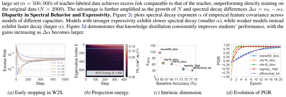
over the course of 5 epochs. Additionally, upon completion of training, we identify the minimum number of dimensions required to account for 80% of the total cumulative energy ( Pk j=1 |⟨wS,uj ⟩|2 P768 j=1 |⟨wS,uj ⟩|2 ≥0.8). Calculate k90%.In Figure 3c and Figure 3d we choose a 50,000 subset of the test set of ImageNet(Deng et al., 2009) and split it into...
2009
discussion (0)
Sign in with ORCID, Apple, or X to comment. Anyone can read and Pith papers without signing in.