Fracton Topological Holography
Pith reviewed 2026-06-28 10:10 UTC · model grok-4.3
The pith
Fracton topological holography extends the bulk-boundary realization of symmetries and dualities to both type-I and type-II fracton stabilizer codes.
A machine-rendered reading of the paper's core claim, the machinery that carries it, and where it could break.
Core claim
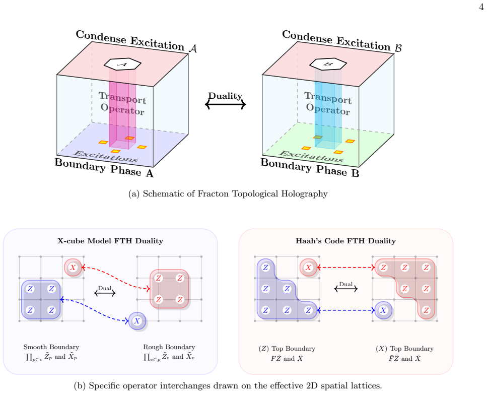
Fracton topological holography is realized by preparing the bulk fracton stabilizer code, computing its excitations, determining admissible gapped top boundaries, identifying the low-energy preserving operator algebra together with its symmetry, relation, and twist data, and then switching among top boundaries to compare the induced boundary descriptions. For the X-cube model both smooth and rough boundaries yield transverse-field plaquette Ising models whose subsystem symmetry and twist data are exchanged, with the boundary switch implemented by a linear-depth local unitary sequential quantum circuit. For Haah's cubic code the natural (Z) and (X) top boundaries induce two two-dimensional qu
What carries the argument
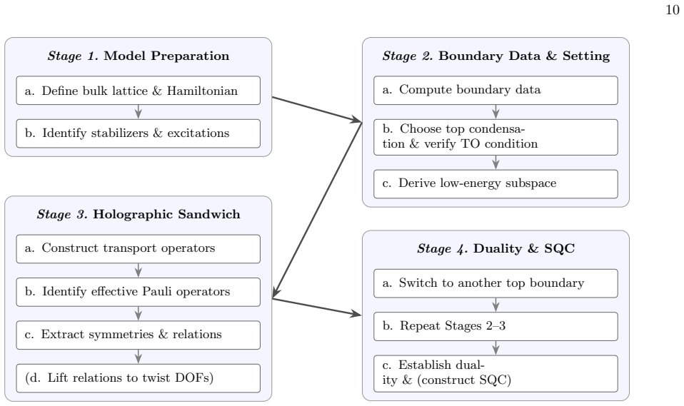
The four-stage framework that uses bulk excitations of a fracton stabilizer code to fix admissible gapped top boundaries and the associated low-energy operator algebra.
If this is right
- FTH applies to both type-I fracton orders such as the X-cube model and type-II orders such as Haah's cubic code.
- Boundary switches for the X-cube model are realized by linear-depth local unitary sequential quantum circuits.
- The construction produces explicit dual pairs of boundary theories in which symmetries and twist data are exchanged.
- FTH supplies a concrete framework for organizing duality in fracton orders and offers a systematic route to new dualities.
Where Pith is reading between the lines
- The same bulk-boundary procedure may be applied to fracton models that are not stabilizer codes.
- The framework could be used to search for previously unknown dualities among three-dimensional codes with restricted mobility.
- Sequential quantum circuits that implement boundary switches may be relevant for quantum simulation protocols involving fracton phases.
Load-bearing premise
Bulk excitations of a fracton stabilizer code determine admissible gapped top boundaries and the low-energy operator algebra in direct analogy with liquid topological orders.
What would settle it
A calculation for the X-cube model showing that the operator algebra on the rough boundary does not reproduce the transverse-field plaquette Ising model with the predicted exchanged subsystem symmetry and twist data.
Figures
read the original abstract
Topological holography (TH), or SymTFT, realizes symmetries and dualities of a quantum system as boundary data of a topological bulk in one higher dimension. We formulate fracton topological holography (FTH), extending this mechanism from liquid topological orders to fracton stabilizer codes. The construction is organized as a general four-stage framework: prepare the bulk model and compute its excitations, determine boundary data and admissible gapped top boundaries, identify the low-energy preserving operator algebra together with its symmetry, relation, and twist data, and then switch among top boundaries to compare the induced boundary descriptions. As a type-I example, we develop FTH for the X-cube model with smooth and rough top boundaries; for a minimal effective Hamiltonian, both yield transverse-field plaquette Ising models, with exchanged subsystem symmetry and twist data, and the boundary switch is implemented by a linear-depth local unitary sequential quantum circuit (SQC). As a type-II example, we formulate FTH for Haah's cubic code in the Laurent-polynomial stabilizer formalism and analyze the natural $(Z)$ and $(X)$ top boundaries, which induce two two-dimensional qubit systems related locally by exchanging generalized plaquette Ising and transverse-field terms and nonlocally by a symmetry--relation duality. These results show that FTH is a genuine extension of TH to both type-I and type-II fracton orders. FTH therefore provides a concrete framework for organizing and understanding duality, with the prospect of offering a systematic route to new dualities.
Editorial analysis
A structured set of objections, weighed in public.
Referee Report
Summary. The paper formulates fracton topological holography (FTH) as an extension of topological holography (SymTFT) to fracton stabilizer codes via a four-stage framework: prepare bulk model and compute excitations, determine boundary data and admissible gapped top boundaries, identify low-energy preserving operator algebra with symmetry/relation/twist data, and switch among top boundaries. Explicit constructions are given for the X-cube model (type-I), where smooth/rough boundaries map to transverse-field plaquette Ising models with exchanged subsystem symmetry and twist data via a linear-depth local unitary sequential quantum circuit, and for Haah's cubic code (type-II) in the Laurent-polynomial formalism, where (Z) and (X) boundaries induce two 2D qubit systems related by local term exchange and nonlocal symmetry-relation duality. The results are presented as showing FTH is a genuine extension providing a framework for organizing dualities in fracton orders.
Significance. If the central constructions and boundary classifications hold with full derivations, FTH would extend the SymTFT paradigm to both type-I and type-II fracton orders, supplying concrete examples of duality organization and a potential systematic route to new dualities; the explicit X-cube SQC boundary switch and Haah's code term-exchange mapping are strengths that could be built upon if verified.
major comments (3)
- [Abstract] Abstract, four-stage framework description: the assumption that the spectrum of bulk excitations (including subdimensional fractons) directly classifies admissible gapped top boundaries and the associated low-energy preserving operator algebra in direct analogy with liquid topological orders is load-bearing for the extension claim, yet no general derivation is supplied showing why subdimensional mobility does not obstruct the classification or require extra foliation data.
- [X-cube construction] X-cube example (smooth/rough boundaries): the claim that both yield transverse-field plaquette Ising models with exchanged subsystem symmetry and twist data, with the boundary switch realized by a linear-depth local unitary SQC, is central to demonstrating the framework but rests on sketched mappings without the explicit operator-algebra derivations, error analysis, or verification steps needed to confirm the low-energy equivalence.
- [Haah's code analysis] Haah's cubic code (Laurent-polynomial formalism, (Z) and (X) boundaries): the mapping to two 2D systems related locally by exchanging generalized plaquette Ising and transverse-field terms and nonlocally by a symmetry-relation duality is presented as supporting the type-II extension, but lacks the detailed identification of the low-energy preserving operator algebra and admissible boundary data required to substantiate the four-stage framework beyond the liquid-order case.
Simulated Author's Rebuttal
We thank the referee for their thorough review and valuable comments. We address each major comment in turn, providing clarifications and indicating where revisions will be made to strengthen the manuscript.
read point-by-point responses
-
Referee: [Abstract] Abstract, four-stage framework description: the assumption that the spectrum of bulk excitations (including subdimensional fractons) directly classifies admissible gapped top boundaries and the associated low-energy preserving operator algebra in direct analogy with liquid topological orders is load-bearing for the extension claim, yet no general derivation is supplied showing why subdimensional mobility does not obstruct the classification or require extra foliation data.
Authors: The four-stage framework is introduced as a direct extension of the SymTFT approach, adapted to the stabilizer formalism for fracton orders. While we do not provide a general mathematical derivation proving that subdimensional mobility does not require additional foliation data, the framework is validated through explicit constructions in the X-cube and Haah's code examples, where the boundary data and operator algebras are identified without obstruction. We will revise the abstract and introduction to clarify that the classification is demonstrated via these examples rather than claimed as a general theorem. revision: partial
-
Referee: [X-cube construction] X-cube example (smooth/rough boundaries): the claim that both yield transverse-field plaquette Ising models with exchanged subsystem symmetry and twist data, with the boundary switch realized by a linear-depth local unitary SQC, is central to demonstrating the framework but rests on sketched mappings without the explicit operator-algebra derivations, error analysis, or verification steps needed to confirm the low-energy equivalence.
Authors: In the manuscript, the mappings are derived using the stabilizer formalism, showing the explicit correspondence to the transverse-field plaquette Ising models and the action of the SQC. To enhance clarity, we will include additional details on the operator algebra derivations and verification of low-energy equivalence in a revised version, possibly in an appendix. revision: yes
-
Referee: [Haah's code analysis] Haah's cubic code (Laurent-polynomial formalism, (Z) and (X) boundaries): the mapping to two 2D systems related locally by exchanging generalized plaquette Ising and transverse-field terms and nonlocally by a symmetry-relation duality is presented as supporting the type-II extension, but lacks the detailed identification of the low-energy preserving operator algebra and admissible boundary data required to substantiate the four-stage framework beyond the liquid-order case.
Authors: The analysis for Haah's code uses the Laurent-polynomial formalism to identify the boundary-induced systems and the duality. We will expand the section to provide more explicit details on the low-energy preserving operator algebra and the admissible boundary data, ensuring the four-stage framework is fully substantiated for the type-II case. revision: yes
Circularity Check
No significant circularity; explicit construction for specific models
full rationale
The paper defines a four-stage framework and applies it explicitly to the X-cube model and Haah's code, deriving specific boundary theories (plaquette Ising models with exchanged data, and term-exchanged systems with duality). No steps reduce by construction to inputs, no self-citations are load-bearing in the provided text, and the derivation is self-contained as a construction rather than a prediction forced by fitting or definition. The analogy to liquid orders is an explicit assumption, not a hidden tautology.
Axiom & Free-Parameter Ledger
axioms (1)
- domain assumption Bulk excitations determine admissible gapped top boundaries and the low-energy operator algebra in the same manner as for liquid topological orders.
Reference graph
Works this paper leans on
-
[1]
(8), i.e
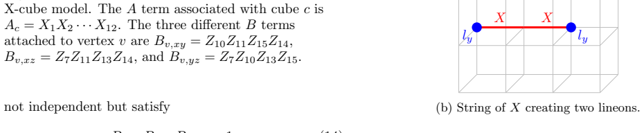
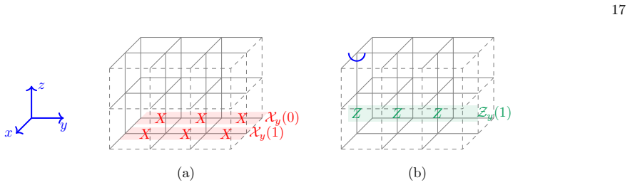
with smooth top boundary (mparticle condensed) Let us start from Eq. (8), i.e. HT H =−η X stabilizers + ˜H . When the top boundary is smooth, the stabilizers are (1) theB v terms associated with all the crossed vertices in Fig. 13, i.e. all theB v terms except those associated with the vertices on the bottom boundary and the hollowed vertex in Fig. 13; (2...
-
[2]
˜Xi+1/2, ˜Zi+1/2 both commute with all stabilizers, so that ˜Xi+1/2, ˜Zi+1/2 map ˜Hto itself
-
[3]
˜Xi+1/2, ˜Zi+1/2 generate the full 2×2 matrix algebraM 2(C) ∼= B( ˜H1+1/2)
-
[4]
4.∀i̸=j, h B( ˜Hi+1/2),B( ˜Hj+1/2) i = 0, i.e
˜Xi+1/2, ˜Zi+1/2 are local alongx-direction, so eachB( ˜Hi+1/2) is local alongx-direction. 4.∀i̸=j, h B( ˜Hi+1/2),B( ˜Hj+1/2) i = 0, i.e. operators acting on ˜Hi+1/2 and ˜Hj+1/2 are commutable. From Eq. (A1) it can be seen that conditions 1,3 and 4 are true. As for condition 2, ˜Xi+1/2, ˜Zi+1/2 indeed generate the full 2×2 matrix algebraM 2(C) ∼= B( ˜Hi+1...
-
[5]
(A5) or Fig
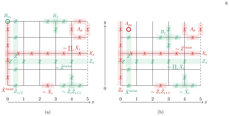
The exception is that wheni=− 1 2 modL x, sinceA v0 ∼ ˜Ztwist [see Eq. (A5) or Fig. 2 (a)] is not a stabilizer, we have the following operator identification, Bv0 ∼ ˜Ztwist Z Z Z Z ∼ ˜Z1/2 Z Z Z Z ∼ ˜Z−1/2 ∼ Z Z Z ∼ ˜Z1/2 ˜Z−1/2 ˜Ztwist , (A5) 34 Twist can be discussed only after we choose the specific low-energy Hamiltonian ˜Hin Eq. (9) [or equivalently,...
-
[6]
2 (b)] is also given by log 2 dim ˜H=L x + 1
with rough top boundary (eparticle condensed) On the other side, it can be calculated that the dimension of low-energy subspace ˜Hwhen the top boundary is rough [with an omittedA p term as shown in Fig. 2 (b)] is also given by log 2 dim ˜H=L x + 1. Then, it can be shown that ˜Hcan be decomposed into ˜HtwistNLx i=1 ˜Hi, where ˜Htwist ∼= ˜Hi ∼= C2. Each ˜Hi...
-
[7]
(B8), we get dim(imV s) =|RS|.(B9) Take Eq
According to rank-nullity theorem, dim(imV P ) + dim(kerVP ) = dim(domainV P ) =|S|,(B7) dim(imV s) + dim(kerVs) = dim(domainV s) =|RS|.(B8) We have supposed thatRSis an independent set of stabilizer redundancies, which means kerVs ={0}, dim(kerV s) = 0, take it into Eq. (B8), we get dim(imV s) =|RS|.(B9) Take Eq. (B6) into Eq. (B7), we get dim(imV P ) + ...
-
[8]
B to compute the dimension of the low-energy subspace ˜H, i.e
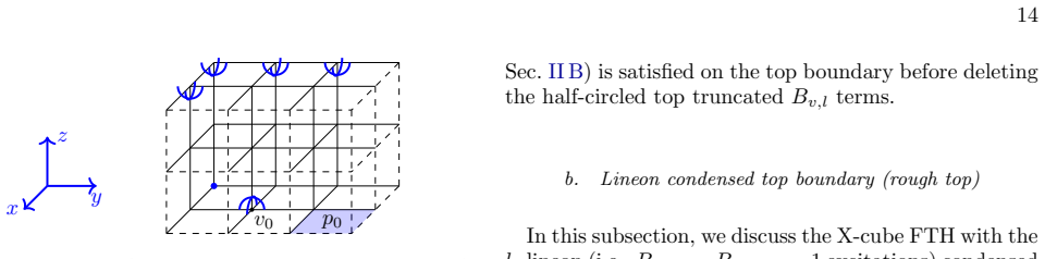
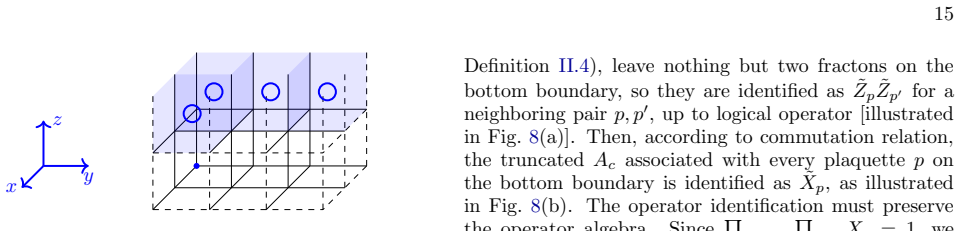
under planeon condensed top boundary In this subsection, we use the higher-order redundancy theory introduced in Appendix. B to compute the dimension of the low-energy subspace ˜H, i.e. the common +1 eigenspace of all the stabilizers 1 of the X-cube FTH under planeon condensed top boundary. The lattice and stabilizer setting follow Sec. III B a. For clari...
-
[9]
B to compute the dimension of the low-energy subspace ˜H, i.e
under lineon condensed top boundary In this subsection, we use the higher-order redundancy theory introduced in Appendix. B to compute the dimension of the low-energy subspace ˜H, i.e. the common +1 eigenspace of all the stabilizers, under the lineon condensed top boundary. The lattice and stabilizer setting follow from Sec. III B b. For clarity, we start...
-
[10]
Appendix D: Details of operator identification and redundant DOFs of X-cube FTH
+ (Lx +L y −1−1) =L xLy +L x +L y + 2Lz, which is the same as the dim ˜Hof X-cube FTH onL x ×L y ×L z lattice with smooth top boundary. Appendix D: Details of operator identification and redundant DOFs of X-cube FTH
-
[11]
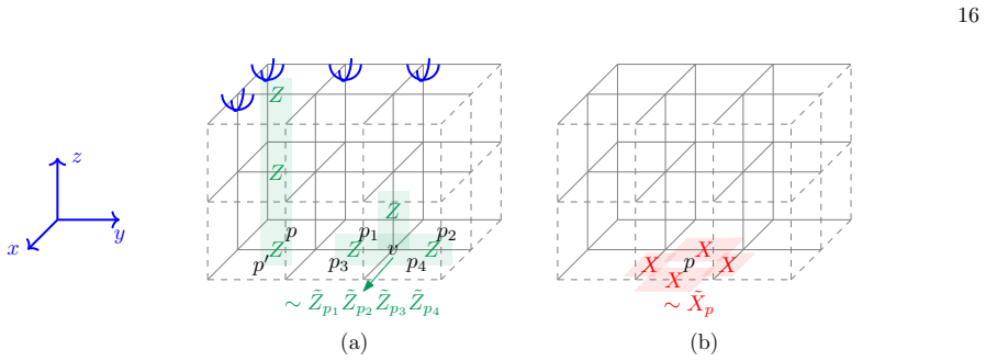
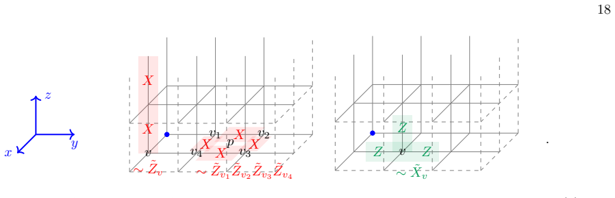
Under planeon condensed top boundary a. Twist logical operator and twist indicator.The identification of twist logical operators are: B[i,j,Lz],xz ∼B [i,j,Lz],yz ∼ ˜Ztwist(i, j), i∈Z Lx , j∈Z Ly ,0∈ {i, j}.(D1) HereB [i,j,Lz],xz ∼B [i,jLz],yz means differ by a multiplication of stabilizer, whileB [i,j,Lz],yz ∼ ˜Ztwist(i, j) means the twist logical operato...
-
[12]
Under lineon condensed top boundary Similarly, the explicit coordinate constraints for the lineon condensed boundary are: Y e⊂[i+1/2,j+1/2,0] Xe ∼ Y v⊂[i+1/2,j+1/2] ˜Zv, i∈Z Lx , j∈Z Ly , i̸= 0, j̸= 0,(D11) Y e⊂[i+1/2,j+1/2,0] Xe ∼ Y v⊂[i+1/2,j+1/2] ˜Zv · ˜Ztwist(i+ 1/2, j+ 1/2), i∈Z Lx , j∈Z Ly ,0∈ {i, j}.(D12) as defined in Eq. (24). We illustrate ˜Ztwi...
-
[13]
[48], wherepwas assumed to be prime
Pedagogical review of the translation-invariant stabilizer code formalism In this Appendix, we review the formalism of translational-invariantZ p stabilizer code introduced by Haah in Ref. [48], wherepwas assumed to be prime. Later, the formalism was generalized to the cases where the qudit dimension could be non-prime[87]. We focus on the primepcases in ...
-
[14]
Choose a basis of the free moduleR 2q that correspond to single PauliX, Zof the system: X1 ≡X (0,0),1 := (1,0,· · ·,0; 0,0,· · ·,0) T ,· · · · · ·, X q ≡X (0,0),q := (0,0,· · ·,1; 0,0,· · ·,0) T , Z1 ≡Z (0,0),1 := (0,0,· · ·,0; 1,0,· · ·,0) T ,· · · · · ·, Z q ≡Z (0,0),q := (0,0,· · ·,0; 0,0,· · ·,1) T ,(E3) whereX (0,0),α is theα-th qudit in the cell at ...
-
[15]
Let xiyjX(0,0),α ≡X (i,j),α,(E4) whereX (i,j),α is theα-th qudit in the cell at (i, j)
-
[16]
For example, (1 +x 2,0,· · ·,¯y; 2x,0,· · ·,0) T corresponds to X(0,0),1X(2,0),1X(0,−1),qZ2 (1,0),1
According toR-linearity, other elements inR 2q can be read. For example, (1 +x 2,0,· · ·,¯y; 2x,0,· · ·,0) T corresponds to X(0,0),1X(2,0),1X(0,−1),qZ2 (1,0),1. Here ¯y≡y −1. Similarly, ¯x≡x −1. For anyu= P ij uijxiyj ∈R, ¯u≡ P ij uij ¯xi¯yj. Like before, the commutation phase information can be encoded into a bilinear symplectic form Ω :R 2q ×R 2q →R, re...
-
[17]
When the commutation relation we are talking about only involves qubits in some specific layers, we can use the symplectic bilinear form in the corresponding Pauli submodule
Layer-by-layer bulk syndrome and stabilizer representation To facilitate analysis near the boundaries, we separate the stabilizer moduleS B, the truncated Pauli moduleπP, and the bulk excitation moduleE B into layer-by-layer submodules: SB = Lz−1M k=0 Sk+1/2, πP= Lz−1M k=0 Pk, E B = Lz−2M k=0 Ek+1/2, whereP k ∼= R4 is the Pauli submodule of qubits in thez...
-
[18]
Boundary gauge operators, syndromes and boundary topological excitations a. Bottom boundary By convention, take the following basis for bottom boundary gauge syndrome moduleG bot, Gbot 1 := 1 0 ! ,G bot 2 := 0 1 ! ,(E11) whereG bot 1,2 are the bottom truncated stabilizers, defined in Eq. (63).G bot 1,2 only involve Pauli operators inP 0, so P bot =P 0 = s...
-
[19]
Denote theR-module of possibly infinite support series ˆR:=F 2[[x±1, y±1]],(E38) so that the possibly infinite support Pauli operators form theR-module ˆP ∼= ˆR4Lz
Point-like excitations via infinite support operators Now we show singlee bot X and singlee bot Z can be created by infinite support Pauli operators 1, so they are indeed point-like bottom boundary topological excitations. Denote theR-module of possibly infinite support series ˆR:=F 2[[x±1, y±1]],(E38) so that the possibly infinite support Pauli operators...
-
[20]
Lemma E.1.Under(Z)top boundary, S(Z) +G bot Ω =S (Z)
No nontrivial finite-support logical operator In this appendix, we place some of the theorems/lemmas and proofs in the study of Haah’s code FTH. Lemma E.1.Under(Z)top boundary, S(Z) +G bot Ω =S (Z). 1By definition, the support of an operatorOis the set of all (i, j)∈Z 2 whereOacts nontrivially on. An operatorOis called finite support if∃r∈N, s.t. supp(O)⊂...
-
[21]
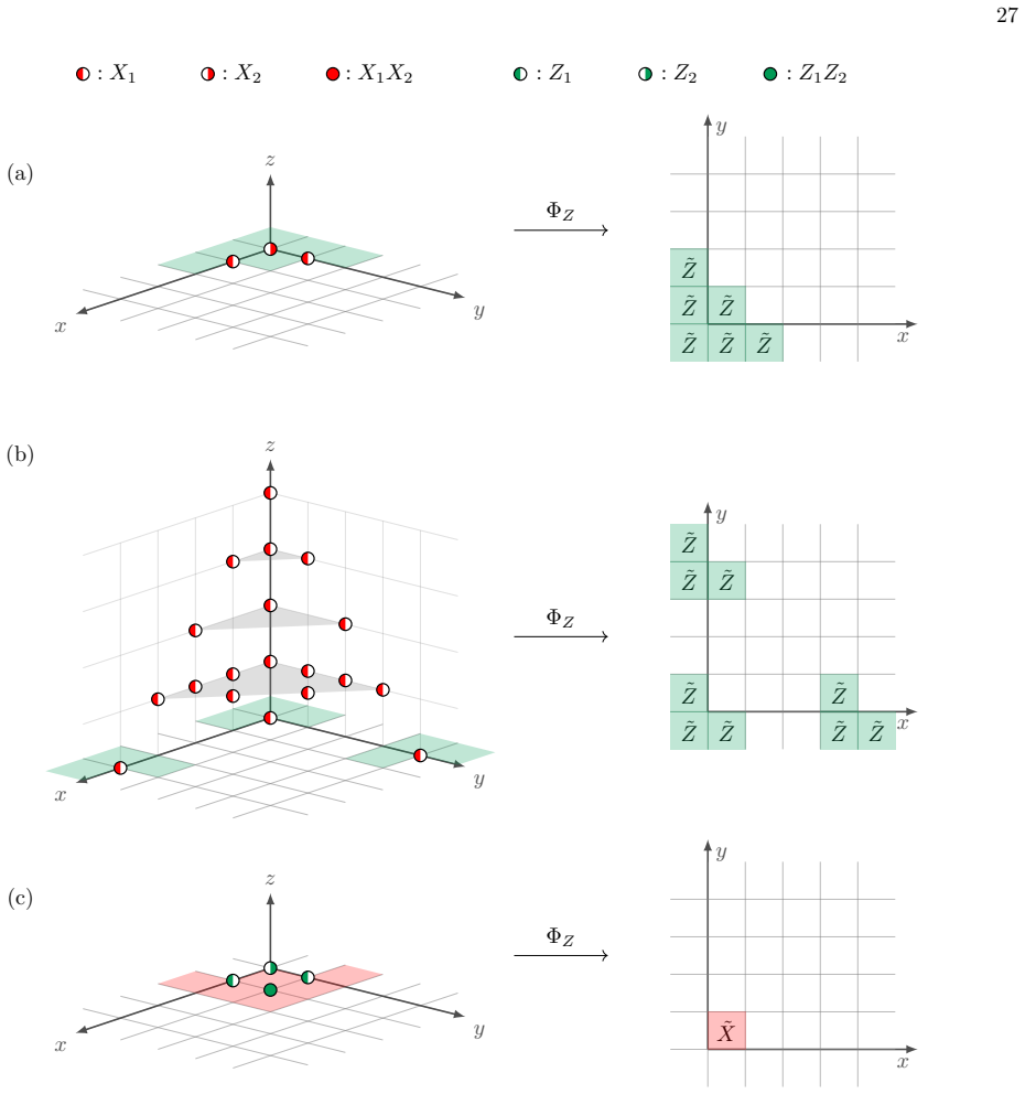
We first derive the general form of low-energy preserving Pauli operators, i.e
Generators of low-energy preserving operator module under(Z)top boundary In this Appendix, we derive the generators of low-energy preserving operator module under (Z) top boundary, namely,O (Z). We first derive the general form of low-energy preserving Pauli operators, i.e. elements inS Ω (Z); then we prove that two low-energy preserving Pauli operators w...
-
[22]
Using gcd(A, B) = 1 and Theorem E.5, we getA|g (0) 2 andB|g (0) 1
Denote g(1) 1 :=u 1 +DU 1/2 +Dw 1, g (1) 2 :=v 1 +U 1/2 +w 1, we get Ag(1) 1 +Bg (1) 2 = 0⇐ ⇒Ag (1) 1 =Bg (1) 2 =⇒A|Bg (1) 2 &B|Ag (1) 1 . Using gcd(A, B) = 1 and Theorem E.5, we getA|g (0) 2 andB|g (0) 1 . Combining withAg (1) 1 =Bg (1) 2 , we get g(1) 1 =BU 3/2, g (1) 2 =AU 3/2, for someU 3/2 ∈R. 3.g (1) 1 , g(1) 2 are theX 1, X2 coefficients ofδO (1) X...
-
[23]
This can be iteratively done, until we get δO(Lz−1) X :=δO (Lz−2) X +xyz Lz−2SX ULz−3/2 =xyz Lz−1Gbot 1 ULz−3/2 +δO X,Lz−1, which has support only in thez=L z −1 top layer
Recall that SX = ¯x¯y xyzG bot 1 + ¯z(BX1 +AX 2) , 53 we have δO(2) X :=δO (1) X +xyzS X U3/2 =xyz 2Gbot 1 U3/2 + Lz−1X k=2 δOX,k, which has no support in thez= 0,1 layers. This can be iteratively done, until we get δO(Lz−1) X :=δO (Lz−2) X +xyz Lz−2SX ULz−3/2 =xyz Lz−1Gbot 1 ULz−3/2 +δO X,Lz−1, which has support only in thez=L z −1 top layer. The final s...
-
[24]
Using gcd(A, B) = 1 and Theorem E.5, we getA|g (Lz−1) 2 andB|g (Lz−1) 1
Denote g(Lz−1) 1 :=u Lz−1 +DU Lz−3/2 +Dw Lz−1, g (Lz−1) 2 :=v Lz−1 +U Lz−3/2 +w Lz−1, so that the no bulk syndrome condition ofδO (Lz−1) X can be written as Ag(Lz−1) 1 +Bg (Lz−1) 2 = 0⇐ ⇒Ag (Lz−1) 1 =Bg (Lz−1) 2 =⇒A|Bg (Lz−1) 2 &B|Ag (Lz−1) 1 . Using gcd(A, B) = 1 and Theorem E.5, we getA|g (Lz−1) 2 andB|g (Lz−1) 1 . Combining withAg (Lz−1) 1 =Bg (Lz−1) 2...
-
[25]
differing by a stabilizer
Recall that Gtop 1 = ¯x¯yzLz−2(BX1 +AX 2). Gtop 1 is a stabilizer on the (Z) top boundary. δO(Lz) X :=δO (Lz−1) X +xyG top 1 ULz−1/2 = 0. In all, δO(Lz) X =δO X + Lz−2X k=0 xyz kSX ULz−3/2 +xyG top 1 ULz−1/2 = 0, δOX is a stabilizer,O X andO ′ X differ by a stabilizer.QED. Clear the definition ofu k,v k,r k+1/2,t k,g (k) 1 ,g (k) 2 ,U k+1/2, they will be ...
-
[26]
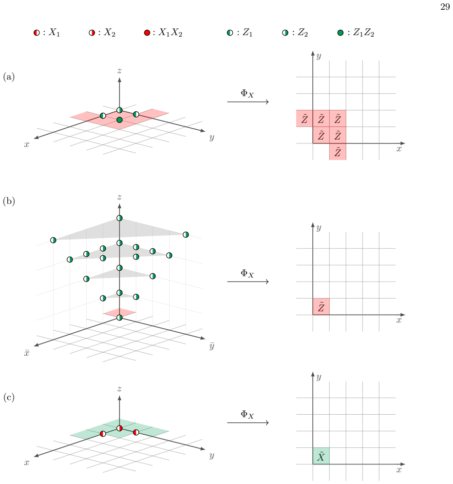
We first derive the general form of low-energy preserving Pauli operators, i.e
Generators of low-energy preserving operator module under(X)top boundary In this Appendix, we derive the generators of low-energy preserving operators module under (X) top boundary, namely,O (X). We first derive the general form of low-energy preserving Pauli operators, i.e. elements inS Ω (X); then we prove that two low-energy preserving operators with t...
-
[27]
56 Supposeg (1) 2 =DU 3/2, taking it back toDg (1) 1 =xyg (1) 2 , we getDg (1) 1 =xyDU 3/2, which impliesg (1) 1 =xyU 3/2 sinceRis a UFD
Denote g(1) 1 :=xy ¯AU1/2 +u 1, g (1) 2 :=BU 1/2 +v 1, we get Dg(1) 1 +xyg (1) 2 = 0⇐ ⇒Dg (1) 1 =xyg (1) 2 =⇒D|g (1) 2 . 56 Supposeg (1) 2 =DU 3/2, taking it back toDg (1) 1 =xyg (1) 2 , we getDg (1) 1 =xyDU 3/2, which impliesg (1) 1 =xyU 3/2 sinceRis a UFD. 3.g (1) 1 , g(1) 2 are theZ 1, Z2 coefficients ofδO (1) Z in thez= 1 layer. Therefore, δO(1) Z =g ...
-
[28]
This can be iteratively done, until we get δO(Lz−1) Z :=δO (Lz−2) Z +xyz Lz−2SX ULz−3/2 =z Lz−2(xy ¯AZ1 +BZ 2)ULz−3/2 +δO X,Lz−1, which has support only in thez=L z −1 top layer
Using xySZ = ¯z(xyZ1 +DZ 2) +xy ¯AZ1 +BZ 2, we can write δO(2) Z :=δO (1) Z +xyzS ZU3/2 =z(xy ¯AZ1 +BZ 2)U3/2 + Lz−1X k=2 δOX,k, which has no support in thez= 0,1 layers. This can be iteratively done, until we get δO(Lz−1) Z :=δO (Lz−2) Z +xyz Lz−2SX ULz−3/2 =z Lz−2(xy ¯AZ1 +BZ 2)ULz−3/2 +δO X,Lz−1, which has support only in thez=L z −1 top layer. The fin...
-
[29]
Supposeg (Lz−1) 2 =DU Lz−1/2, taking it back toDg (Lz−1) 1 =xyg (Lz−1) 2 , we getDg (Lz−1) 1 =xyDU Lz−1/2, which impliesg (Lz−1) 1 =xyU Lz−1/2 sinceRis a UFD
Denote g(Lz−1) 1 :=xy ¯AULz−3/2 +u Lz−1, g (Lz−1) 2 :=BU Lz−3/2 +v Lz−1, we get Dg(Lz−1) 1 +xyg (Lz−1) 2 = 0⇐ ⇒Dg (Lz−1) 1 =xyg (Lz−1) 2 =⇒D|g (Lz−1) 2 . Supposeg (Lz−1) 2 =DU Lz−1/2, taking it back toDg (Lz−1) 1 =xyg (Lz−1) 2 , we getDg (Lz−1) 1 =xyDU Lz−1/2, which impliesg (Lz−1) 1 =xyU Lz−1/2 sinceRis a UFD. 3.g (Lz−1) 1 , g(Lz−1) 2 are theZ 1, Z2 coef...
-
[30]
differing by a stabilizer
Recall that xyGtop 2 =z Lz−2(xyZ1 +DZ 2), so we can write δO(Lz) Z :=δO (Lz−1) Z +xyG top 2 ULz−1/2 = 0. In all, δO(Lz) Z =δO Z + Lz−2X k=0 xyz kSZUk+1/2 +xyG top 2 ULz−1/2 = 0. 57 SinceG top 2 ∈ S(X),δO Z differ from 0 by a stabilizer.O Z, O′ Z differ by a stabilizer.QED. c. Conclusion We have derived in Appendix E 7 a that the bottom syndrome ofZ-type l...
-
[31]
Identification ofotherbottom boundary gauge operators In this Appendix, we illustrate the detailed calculation for settling down the identification ofotherbottom boundary gauge operator generators, whereothermeans the operator’s boundary gauge syndrome is not a sum of top condensed topological excitations, or equivalently, those bottom boundary gauge gene...
-
[32]
LU circuit connectivity forv̸= 0 Under the (Z) top boundary, for a generalv= ¯v, the identified Hamiltonian is ˜H(Z),v :=− X unitm∈R m F ˜Z+ R h( ˜X+v ˜Z) .(E80) 59 v= ¯vmeansvis symmetric under (x, y)→(¯x,¯y), so the general form ofvis v=a 1 + X m∈H am(m+ ¯m),(E81) wherea 1, am ∈F 2, andHis the half space ofZ 2, s.t.H∪ ¯H=Z 2. For example, we can take H=...
-
[33]
Theorem E.5.In a Unique Factorization Domain (UFD), ifAandFare coprime, andF|As, thenF|s
A theorem in unique factorization domain (UFD) and UFD explanation The following is a basic theorem that will be repeatedly used in the proof of Theorem E.3. Theorem E.5.In a Unique Factorization Domain (UFD), ifAandFare coprime, andF|As, thenF|s. Explanation. •A UFD is an integral domainR, s.t. every nonzero nonunit elementa∈Rcan be written as a finite p...
-
[34]
J. D. Jackson,Classical Electrodynamics(John Wiley & Sons, 2021)
2021
-
[35]
H. A. Kramers and G. H. Wannier, Statistics of the two- dimensional ferromagnet. part I, Physical Review60, 252 (1941)
1941
-
[36]
Jordan and E
P. Jordan and E. Wigner, ¨Uber das paulische ¨ aquivalen- zverbot, Zeitschrift f¨ ur Physik47, 631 (1928)
1928
-
[37]
M. E. Peskin, Mandelstam-’t hooft duality in abelian lat- tice models, Annals of Physics113, 122 (1978)
1978
-
[38]
Dasgupta and B
C. Dasgupta and B. I. Halperin, Phase transition in a lat- tice model of superconductivity, Physical Review Letters 47, 1556 (1981)
1981
-
[39]
Wilczek, Magnetic flux, angular momentum, and statistics, Physical Review Letters48, 1144 (1982)
F. Wilczek, Magnetic flux, angular momentum, and statistics, Physical Review Letters48, 1144 (1982)
1982
-
[40]
A. M. Polyakov, Fermi-bose transmutations induced by gauge fields, Modern Physics Letters A3, 325 (1988)
1988
-
[41]
J. K. Jain, Composite-fermion approach for the fractional quantum hall effect, Physical Review Letters63, 199 (1989)
1989
-
[42]
J. Maldacena, The large-nlimit of superconformal field theories and supergravity, International Journal of The- oretical Physics38, 1113 (1999), arXiv:hep-th/9711200
Pith/arXiv arXiv 1999
-
[43]
D. Gaiotto, A. Kapustin, N. Seiberg, and B. Willett, Generalized global symmetries, Journal of High Energy Physics2015, 172 (2015), arXiv:1412.5148 [hep-th]
Pith/arXiv arXiv 2015
-
[44]
T. D. Brennan and S. Hong, Introduction to generalized global symmetries in QFT and particle physics (2023), arXiv:2306.00912 [hep-ph]
arXiv 2023
- [45]
-
[46]
L. Kong, X.-G. Wen, and H. Zheng, Boundary-bulk rela- tion for topological orders as the functor mapping higher categories to their centers (2015), arXiv:1502.01690 [cond-mat.str-el]
Pith/arXiv arXiv 2015
-
[47]
W. Ji and X.-G. Wen, Categorical symmetry and nonin- vertible anomaly in symmetry-breaking and topological phase transitions, Physical Review Research2, 033417 (2020), arXiv:1912.13492 [cond-mat.str-el]
arXiv 2020
-
[48]
L. Kong, T. Lan, X.-G. Wen, Z.-H. Zhang, and H. Zheng, Algebraic higher symmetry and categorical symmetry – a holographic and entanglement view of symmetry, Phys- ical Review Research2, 043086 (2020), arXiv:2005.14178 [cond-mat.str-el]
arXiv 2020
-
[49]
T. Lichtman, R. Thorngren, N. H. Lindner, A. Stern, and E. Berg, Bulk anyons as edge symmetries: Boundary phase diagrams of topologically ordered states, Physical Review B104, 075141 (2021), arXiv:2003.04328 [cond- mat.str-el]
arXiv 2021
-
[50]
A. Chatterjee and X.-G. Wen, Symmetry as a shadow of topological order and a derivation of topological holo- graphic principle, Physical Review B107, 155136 (2023), arXiv:2203.03596 [cond-mat.str-el]
arXiv 2023
- [51]
-
[52]
D. S. Freed, G. W. Moore, and C. Teleman, Topo- 61 logical symmetry in quantum field theory (2022), arXiv:2209.07471 [hep-th]
Pith/arXiv arXiv 2022
- [53]
- [54]
-
[55]
L. Bhardwaj and S. Sch¨ afer-Nameki, Generalized charges, part II: Non-invertible symmetries and the symmetry TFT, SciPost Physics19, 098 (2025), arXiv:2305.17159 [hep-th]
arXiv 2025
-
[56]
Y.-H. Lin and S.-H. Shao, Bootstrapping non-invertible symmetries, Physical Review D107, 125025 (2023), arXiv:2302.13900 [hep-th]
arXiv 2023
-
[57]
Y. Choi, Y. Sanghavi, S.-H. Shao, and Y. Zheng, Non- invertible and higher-form symmetries in 2 + 1d lat- tice gauge theories, SciPost Physics18, 008 (2025), arXiv:2405.13105 [cond-mat.str-el]
arXiv 2025
-
[58]
J. Chen, W. Cui, B. Haghighat, and Y.-N. Wang, SymTFTs and duality defects from 6d SCFTs on 4- manifolds, Journal of High Energy Physics2023, 208 (2023), arXiv:2305.09734 [hep-th]
arXiv 2023
-
[59]
Q. Jia, R. Luo, J. Tian, Y.-N. Wang, and Y. Zhang, Symmetry topological field theory for flavor symmetry (2025), arXiv:2503.04546 [hep-th]
arXiv 2025
-
[60]
Y.-H. Lin, M. Okada, S. Seifnashri, and Y. Tachikawa, Asymptotic density of states in 2d CFTs with non- invertible symmetries, Journal of High Energy Physics 2023, 094 (2023), arXiv:2208.05495 [hep-th]
arXiv 2023
-
[61]
L. Kong and H. Zheng, Gapless edges of 2d topological orders and enriched monoidal categories, Nuclear Physics B927, 140 (2018), arXiv:1705.01087 [cond-mat.str-el]
Pith/arXiv arXiv 2018
-
[62]
L. Kong and H. Zheng, A mathematical theory of gapless edges of 2d topological orders. part I, Journal of High En- ergy Physics2020, 150 (2020), arXiv:1905.04924 [cond- mat.str-el]
arXiv 2020
-
[63]
L. Kong and H. Zheng, A mathematical theory of gapless edges of 2d topological orders. part II, Nuclear Physics B 966, 115384 (2021), arXiv:1912.01760 [cond-mat.str-el]
arXiv 2021
-
[64]
L. Kong, X.-G. Wen, and H. Zheng, One dimensional gapped quantum phases and enriched fusion categories, Journal of High Energy Physics2022, 022 (2022), arXiv:2108.08835 [cond-mat.str-el]
arXiv 2022
-
[65]
L. Kong and H. Zheng, Categories of quantum liquids I, Journal of High Energy Physics2022, 070 (2022), arXiv:2011.02859 [cond-mat.str-el]
arXiv 2022
-
[66]
L. Kong and H. Zheng, Categories of quantum liquids II, Communications in Mathematical Physics405, 203 (2024), arXiv:2107.03858 [cond-mat.str-el]
arXiv 2024
-
[67]
R. Xu and Z.-H. Zhang, Categorical descriptions of one-dimensional gapped phases with abelian onsite symmetries, Physical Review B110, 155106 (2024), arXiv:2205.09656 [cond-mat.str-el]
arXiv 2024
- [68]
- [69]
-
[70]
A. Chatterjee and X.-G. Wen, Holographic theory for continuous phase transitions: Emergence and symmetry protection of gaplessness, Physical Review B108, 075105 (2023), arXiv:2205.06244 [cond-mat.str-el]
arXiv 2023
-
[71]
S.-J. Huang and M. Cheng, Topological holography, quantum criticality, and boundary states, SciPost Physics18, 213 (2025), arXiv:2310.16878 [cond-mat.str- el]
arXiv 2025
-
[72]
Y.-Z. You, Z. Bi, A. Rasmussen, K. Slagle, and C. Xu, Wave function and strange correlator of short-range en- tangled states, Physical Review Letters112, 247202 (2014), arXiv:1312.0626 [cond-mat.str-el]
Pith/arXiv arXiv 2014
-
[73]
D. Aasen, R. S. K. Mong, and P. Fendley, Topologi- cal defects on the lattice: I. the ising model, Journal of Physics A: Mathematical and Theoretical49, 354001 (2016), arXiv:1601.07185 [cond-mat.stat-mech]
Pith/arXiv arXiv 2016
- [74]
-
[75]
R. Vanhove, M. Bal, D. J. Williamson, N. Bultinck, J. Haegeman, and F. Verstraete, Mapping topologi- cal to conformal field theories through strange corre- lators, Physical Review Letters121, 177203 (2018), arXiv:1801.05959 [cond-mat.str-el]
Pith/arXiv arXiv 2018
-
[76]
R. Vanhove, L. Lootens, H.-H. Tu, and F. Verstraete, Topological aspects of the critical three-state potts model, Journal of Physics A: Mathematical and Theoret- ical55, 235002 (2022), arXiv:2107.11177 [cond-mat.stat- mech]
arXiv 2022
-
[77]
X. Chen, A. Dua, M. Hermele, D. T. Stephen, N. Tan- tivasadakarn, R. Vanhove, and J.-Y. Zhao, Sequential quantum circuits as maps between gapped phases, Phys- ical Review B109, 075116 (2024), arXiv:2307.01267 [cond-mat.str-el]
arXiv 2024
-
[78]
R. Vanhove, V. Ravindran, D. T. Stephen, X.-G. Wen, and X. Chen, Duality via sequential quantum circuit in the topological holography formalism, Physical Review B 112, 035173 (2025), arXiv:2409.06647 [cond-mat.str-el]
arXiv 2025
-
[79]
Chamon, Quantum glassiness in strongly correlated clean systems: An example of topological overprotection, Physical Review Letters94, 040402 (2005)
C. Chamon, Quantum glassiness in strongly correlated clean systems: An example of topological overprotection, Physical Review Letters94, 040402 (2005)
2005
-
[80]
J. Haah, Local stabilizer codes in three dimensions with- out string logical operators, Physical Review A83, 042330 (2011), arXiv:1101.1962 [quant-ph]
Pith/arXiv arXiv 2011
discussion (0)
Sign in with ORCID, Apple, or X to comment. Anyone can read and Pith papers without signing in.