Ceci n'est pas une Couche de M\'elange: The Meaning of Resolved Turbulent Radiative Mixing
Pith reviewed 2026-06-28 08:50 UTC · model grok-4.3
The pith
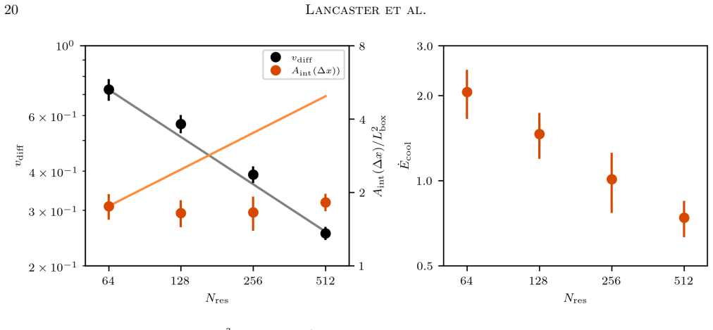
The resolution independence of total cooling in turbulent radiative mixing layer simulations arises from a cancellation between numerical dissipation and numerical viscosity.
A machine-rendered reading of the paper's core claim, the machinery that carries it, and where it could break.
Core claim
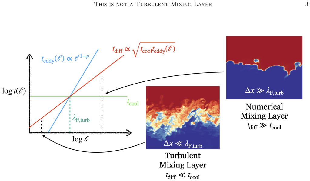
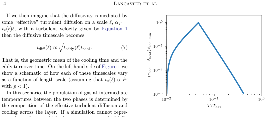
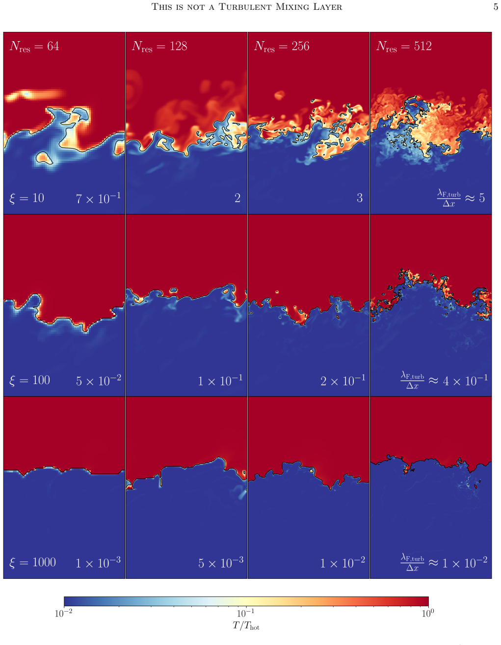
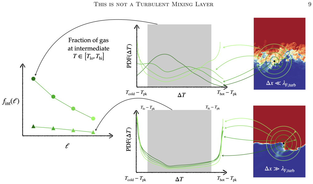
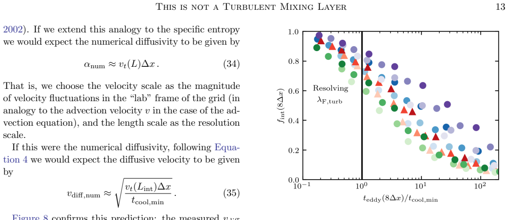
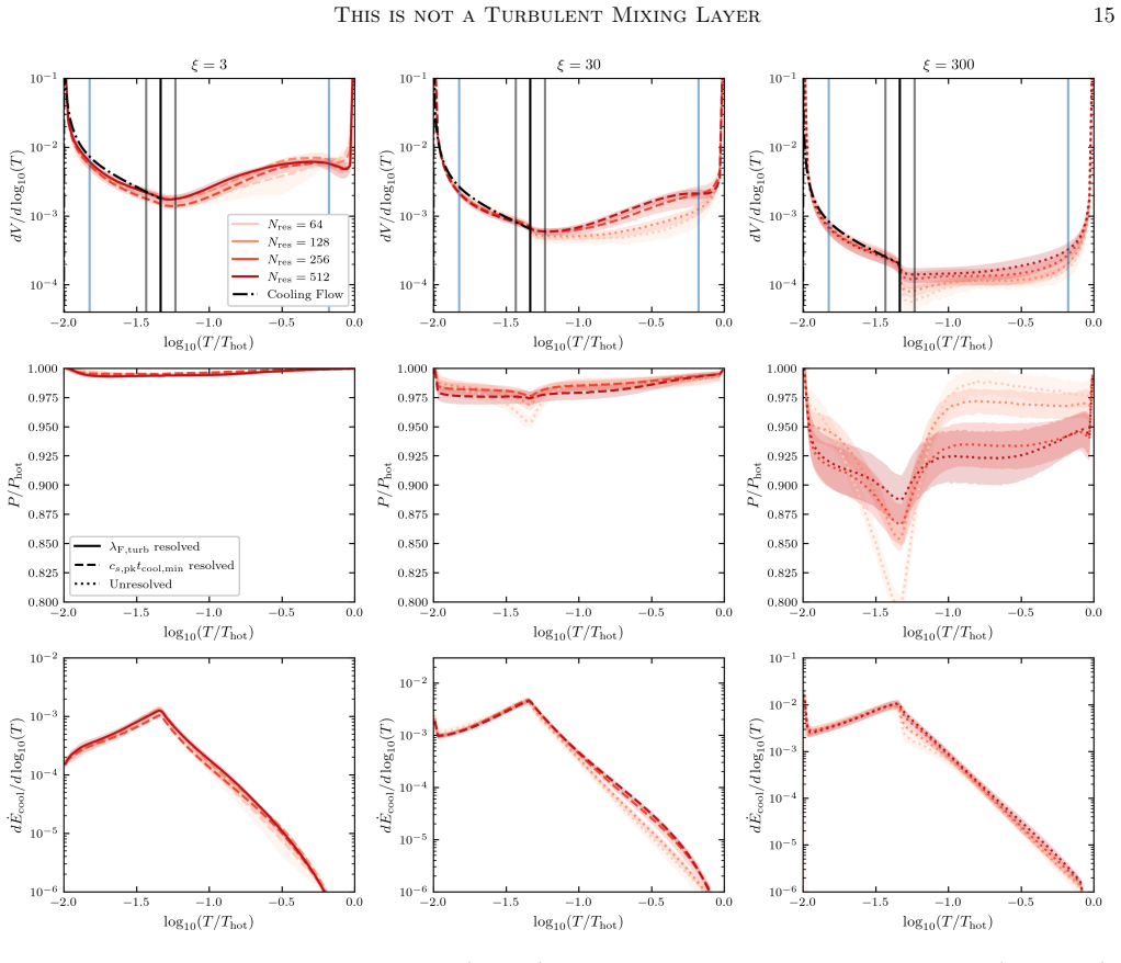
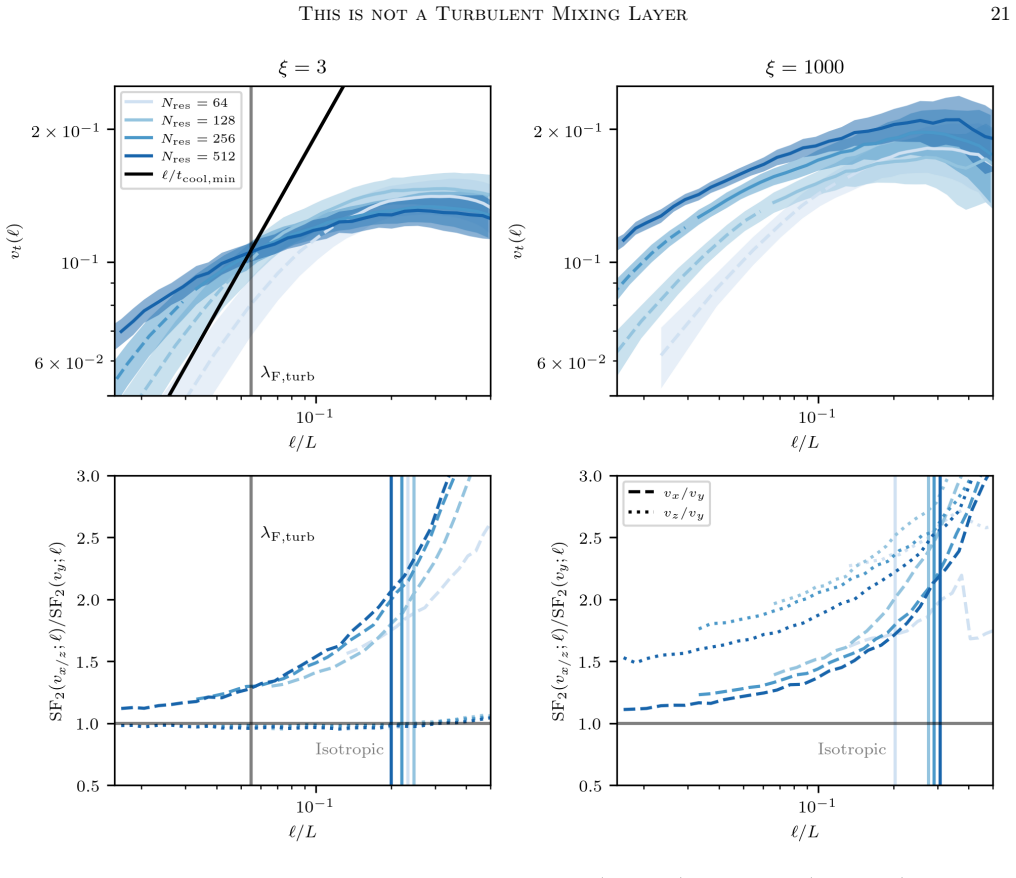
The previously noticed resolution independence of total cooling, Ė_cool, in these simulations is due to a remarkable, and perhaps fortuitous, cancellation of the countervailing effects of numerical dissipation and numerical viscosity. This calls into question the degree to which we can trust the results of these experiments, as there is no physical picture that explains this cancellation. We also demonstrate that in order to correctly resolve the phase structure in these layers, one must resolve the scale on which turbulent diffusion acts on time-scales comparable to the cooling time. This "turbulent Field length", λ_F,turb, is where the eddy turnover time is equal to the cooling time (t_edd
What carries the argument
The turbulent Field length λ_F,turb, defined as the scale where the eddy turnover time equals the cooling time, which must be resolved to capture phase structure correctly.
If this is right
- Total cooling rates may not be physically converged despite appearing resolution-independent.
- Predictions of observable properties depend on resolving the turbulent Field length.
- Simulations need to target the scale where turbulent diffusion time matches cooling time.
- Phase structure in multi-phase fluids requires this resolution criterion.
Where Pith is reading between the lines
- Other astrophysical simulations involving mixing and cooling may suffer similar hidden numerical cancellations.
- Future work could test if the cancellation persists in different codes or setups.
- Defining convergence via the turbulent Field length could become a standard criterion for such problems.
Load-bearing premise
The micro and macro properties measured in the simulations correctly identify the numerical cancellation as the reason for resolution independence of cooling.
What would settle it
A simulation at sufficiently high resolution where the total cooling rate begins to change with further resolution increase, or where phase structure converges only after resolving the turbulent Field length.
Figures
read the original abstract
Turbulent Radiative Mixing Layers (TRMLs) are of fundamental importance to the transport of energy and momentum in multi-phase, astrophysical fluids. We use measurements of the "micro" and "macro" properties of these layers in high-resolution \texttt{AthenaK} simulations to investigate when their properties can be considered \textit{well}-resolved. In particular, we demonstrate that the previously noticed resolution independence of total cooling, $\dot{E}_{\rm cool}$, in these simulations is due to a remarkable, and perhaps fortuitous, cancellation of the countervailing effects of numerical dissipation and numerical viscosity. This calls into question the degree to which we can trust the results of these experiments, as there is no physical picture that explains this cancellation. We also demonstrate that in order to correctly resolve the phase structure in these layers, important for accurate predictions of their observable properties, one must resolve the scale on which turbulent diffusion acts on time-scales comparable to the cooling time. This "turbulent Field length", $\lambda_{\rm F,turb}$, is where the eddy turnover time is equal to the cooling time ($t_{\rm eddy}(\lambda_{\rm F,turb}) = t_{\rm cool}$). We demonstrate that resolving this scale results in converged phase-structure and spatially resolved transitions in the gas phases.
Editorial analysis
A structured set of objections, weighed in public.
Referee Report
Summary. The manuscript uses high-resolution AthenaK simulations of turbulent radiative mixing layers (TRMLs) to examine resolution requirements. It attributes the previously observed resolution independence of total cooling Ė_cool to a cancellation between numerical dissipation (which enhances mixing and cooling) and numerical viscosity (which damps turbulence), and argues this undermines trust in the results absent a physical explanation. It further claims that resolving the turbulent Field length λ_F,turb—defined where the eddy turnover time equals the cooling time (t_eddy(λ_F,turb) = t_cool)—is required for converged phase structure and spatially resolved phase transitions.
Significance. If the central claims hold, the work would caution the community against over-interpreting existing TRML simulation results and introduce a physically motivated resolution criterion tied to turbulent diffusion timescales. The absence of a physical picture for the reported cancellation is already flagged by the authors as a limitation; confirmation via controlled experiments would strengthen the case that current results cannot be trusted at face value.
major comments (3)
- [Abstract] Abstract: the attribution of Ė_cool resolution independence to an exact cancellation between numerical dissipation and numerical viscosity rests on indirect inference from micro- and macro-property measurements; no explicit isolation of the two effects (e.g., via controlled addition of explicit viscosity, changes in Riemann solver, or artificial dissipation runs) is described, leaving the causal link unverified.
- [Abstract] Abstract: the turbulent Field length λ_F,turb is asserted to be the load-bearing scale whose resolution produces converged phase structure, yet no comparative tests against alternative scales (classical Field length, cooling length) or variations in the turbulence driving spectrum and cooling curve are reported to establish uniqueness.
- [Abstract] Abstract: the manuscript provides no quantitative details on error bars, data exclusion criteria, or how the degree of cancellation was measured across resolutions, which weakens the support for the claim that the cancellation is 'remarkable' and resolution-independent.
minor comments (1)
- The manuscript would benefit from a short paragraph in the introduction explaining the Magritte reference in the title for readers outside the immediate subfield.
Simulated Author's Rebuttal
We thank the referee for the careful and constructive review. We respond to each major comment below.
read point-by-point responses
-
Referee: [Abstract] Abstract: the attribution of Ė_cool resolution independence to an exact cancellation between numerical dissipation and numerical viscosity rests on indirect inference from micro- and macro-property measurements; no explicit isolation of the two effects (e.g., via controlled addition of explicit viscosity, changes in Riemann solver, or artificial dissipation runs) is described, leaving the causal link unverified.
Authors: We agree that the link is inferential rather than demonstrated via direct isolation experiments. The manuscript draws the conclusion from trends in micro-property (mixing) and macro-property (total cooling) measurements across resolutions, but does not include controlled runs with added explicit viscosity or solver variations. We will revise the text to state this limitation more explicitly and to frame the cancellation as an observed numerical effect without a physical model. revision: yes
-
Referee: [Abstract] Abstract: the turbulent Field length λ_F,turb is asserted to be the load-bearing scale whose resolution produces converged phase structure, yet no comparative tests against alternative scales (classical Field length, cooling length) or variations in the turbulence driving spectrum and cooling curve are reported to establish uniqueness.
Authors: The definition of λ_F,turb follows directly from equating the local eddy turnover time to the cooling time, which is the relevant timescale for turbulent diffusion to compete with radiative losses. Our results show phase-structure convergence once this scale is resolved. We did not perform the suggested comparative tests or parameter variations in the present study. We will add a discussion section explaining the physical motivation for this particular scale and why alternatives are expected to be less directly relevant, but will not add new simulation suites. revision: partial
-
Referee: [Abstract] Abstract: the manuscript provides no quantitative details on error bars, data exclusion criteria, or how the degree of cancellation was measured across resolutions, which weakens the support for the claim that the cancellation is 'remarkable' and resolution-independent.
Authors: We will expand the methods and results sections to include quantitative details on how the degree of cancellation was assessed, any error estimates used, and the criteria applied to the data across resolutions. revision: yes
Circularity Check
No significant circularity; claims rest on direct simulation measurements
full rationale
The paper derives its claims about Ė_cool resolution independence arising from numerical dissipation-viscosity cancellation and the necessity of resolving λ_F,turb directly from micro/macro property measurements in AthenaK simulations. The turbulent Field length is explicitly defined via t_eddy(λ_F,turb) = t_cool and then shown empirically to produce convergence when resolved, without any reduction of outputs to inputs by construction, fitted parameters renamed as predictions, or load-bearing self-citations. No self-definitional loops, uniqueness theorems imported from prior author work, or ansatzes smuggled via citation appear in the derivation chain. The analysis is therefore self-contained against external simulation benchmarks.
Axiom & Free-Parameter Ledger
axioms (1)
- domain assumption Standard assumptions of compressible fluid dynamics, turbulence, and radiative cooling in astrophysical contexts govern the AthenaK simulations.
invented entities (1)
-
turbulent Field length λ_F,turb
no independent evidence
Reference graph
Works this paper leans on
-
[1]
Abruzzo, M. W., Bryan, G. L., & Fielding, D. B. 2022, ApJ, 925, 199, doi: 10.3847/1538-4357/ac3c48
-
[2]
Abruzzo, M. W., Fielding, D. B., & Bryan, G. L. 2024, ApJ, 966, 181, doi: 10.3847/1538-4357/ad1e51
-
[3]
Armillotta, L., Fraternali, F., Werk, J. K., Prochaska, J. X., & Marinacci, F. 2017, MNRAS, 470, 114, doi: 10.1093/mnras/stx1239
-
[4]
Batchelor, G. K. 1959, Journal of Fluid Mechanics, 5, 113, doi: 10.1017/S002211205900009X
-
[5]
Begelman, M. C., & McKee, C. F. 1990, ApJ, 358, 375, doi: 10.1086/168994 Br¨ uggen, M., & Scannapieco, E. 2016, ApJ, 822, 31, doi: 10.3847/0004-637X/822/1/31 Br¨ uggen, M., Scannapieco, E., & Grete, P. 2023, ApJ, 951, 113, doi: 10.3847/1538-4357/acd63e
-
[6]
Chen, Z., Fielding, D. B., & Bryan, G. L. 2023, ApJ, 950, 91, doi: 10.3847/1538-4357/acc73f
-
[7]
Chen, Z., & Oh, S. P. 2024, MNRAS, 530, 4032, doi: 10.1093/mnras/stae1113
-
[8]
Chernyaev, E. V. 1995, GRAPHICON’95
1995
-
[9]
Constantin, P., Procaccia, I., & Sreenivasan, K. R. 1991, PhRvL, 67, 1739, doi: 10.1103/PhysRevLett.67.1739
-
[10]
Cowie, L. L., & McKee, C. F. 1977, ApJ, 211, 135, doi: 10.1086/154911 Damk¨ ohler, G. 1940, Zeitschrift f¨ ur Elektrochemie und angewandte physikalische Chemie, 46, 601
-
[11]
Das, H. K., & Gronke, M. 2024, MNRAS, 527, 991, doi: 10.1093/mnras/stad3125
-
[12]
Draine, B. T. 2011, Physics of the Interstellar and Intergalactic Medium
2011
-
[13]
2022, MNRAS, 510, 3561, doi: 10.1093/mnras/stab3653
Dutta, A., Sharma, P., & Nelson, D. 2022, MNRAS, 510, 3561, doi: 10.1093/mnras/stab3653
-
[14]
Weisz, D. R. 2019, MNRAS, 490, 1961, doi: 10.1093/mnras/stz2773
-
[15]
Field, G. B. 1965, ApJ, 142, 531, doi: 10.1086/148317
-
[16]
Fielding, D. B., & Bryan, G. L. 2022, ApJ, 924, 82, doi: 10.3847/1538-4357/ac2f41
-
[17]
Fielding, D. B., Ostriker, E. C., Bryan, G. L., & Jermyn, A. S. 2020, ApJL, 894, L24, doi: 10.3847/2041-8213/ab8d2c
-
[18]
1995, Turbulence: The Legacy of A
Frisch, U. 1995, Turbulence: The Legacy of A. N. Kolmogorov (Cambridge University Press)
1995
-
[19]
Grete, P., O’Shea, B. W., & Beckwith, K. 2023, ApJL, 942, L34, doi: 10.3847/2041-8213/acaea7
-
[20]
Gronke, M., & Oh, S. P. 2018, MNRAS, 480, L111, doi: 10.1093/mnrasl/sly131 —. 2020, MNRAS, 492, 1970, doi: 10.1093/mnras/stz3332
-
[21]
R., Jarrod Millman, K., van der Walt, S
Harris, C. R., Jarrod Millman, K., van der Walt, S. J., et al. 2020, arXiv e-prints, arXiv:2006.10256. https://arxiv.org/abs/2006.10256
Pith/arXiv arXiv 2020
-
[22]
Hunter, J. D. 2007, Computing in Science and Engineering, 9, 90, doi: 10.1109/MCSE.2007.55
-
[23]
Jenkins, E. B., & Meloy, D. A. 1974, ApJL, 193, L121, doi: 10.1086/181647
-
[24]
Jennings, R. M., & Li, Y. 2021, MNRAS, 505, 5238, doi: 10.1093/mnras/stab1607
-
[25]
Ji, S., Oh, S. P., & Masterson, P. 2019, MNRAS, 487, 737, doi: 10.1093/mnras/stz1248
-
[26]
2013, ApJ, 779, 48, doi: 10.1088/0004-637X/779/1/48
Kim, J.-G., & Kim, W.-T. 2013, ApJ, 779, 48, doi: 10.1088/0004-637X/779/1/48
-
[27]
2004, ApJL, 602, L25, doi: 10.1086/382478
Koyama, H., & Inutsuka, S.-i. 2004, ApJL, 602, L25, doi: 10.1086/382478
-
[28]
Kritsuk, A. G., Norman, M. L., Padoan, P., & Wagner, R. 2007, ApJ, 665, 416, doi: 10.1086/519443
-
[29]
K.-y., & Acharya, R
Kuo, K. K.-y., & Acharya, R. 2012, Fundamentals of turbulent and multiphase combustion (John Wiley & Sons)
2012
-
[30]
Bryan, G. L. 2024, ApJ, 970, 18, doi: 10.3847/1538-4357/ad47f6
-
[31]
Lancaster, L., Ostriker, E. C., Kim, J.-G., & Kim, C.-G. 2021a, ApJ, 914, 89, doi: 10.3847/1538-4357/abf8ab —. 2021b, ApJ, 914, 90, doi: 10.3847/1538-4357/abf8ac
-
[32]
Lewiner, T., Lopes, H., Vieira, A. W., & and, G. T. 2003, Journal of Graphics Tools, 8, 1, doi: 10.1080/10867651.2003.10487582 24Lancaster et al
-
[33]
Li, Z., Hopkins, P. F., Squire, J., & Hummels, C. 2020, MNRAS, 492, 1841, doi: 10.1093/mnras/stz3567
-
[34]
Lorensen, W. E., & Cline, H. E. 1987, in Proceedings of the 14th Annual Conference on Computer Graphics and Interactive Techniques, SIGGRAPH ’87 (New York, NY, USA: Association for Computing Machinery), 163–169, doi: 10.1145/37401.37422
-
[35]
2020, MNRAS, 494, 2641, doi: 10.1093/mnras/staa812
Mandelker, N., Nagai, D., Aung, H., et al. 2020, MNRAS, 494, 2641, doi: 10.1093/mnras/staa812
-
[36]
Marin-Gilabert, T., Gronke, M., & Oh, S. P. 2025, arXiv e-prints, arXiv:2504.15345, doi: 10.48550/arXiv.2504.15345
work page internal anchor Pith review Pith/arXiv arXiv doi:10.48550/arxiv.2504.15345 2025
-
[37]
P., O’Leary, R., & Madigan, A.-M
McCourt, M., Oh, S. P., O’Leary, R., & Madigan, A.-M. 2018, MNRAS, 473, 5407, doi: 10.1093/mnras/stx2687
-
[38]
2025, arXiv e-prints, arXiv:2511.00229, doi: 10.48550/arXiv.2511.00229
Mohapatra, R., Dutta, A., & Sharma, P. 2025, arXiv e-prints, arXiv:2511.00229, doi: 10.48550/arXiv.2511.00229
-
[39]
2023, MNRAS, 525, 3831, doi: 10.1093/mnras/stad2574
Mohapatra, R., Sharma, P., Federrath, C., & Quataert, E. 2023, MNRAS, 525, 3831, doi: 10.1093/mnras/stad2574
-
[40]
2013, Statistical Fluid Mechanics, Volume II: Mechanics of Turbulence, Dover Books on Physics (Dover Publications)
Monin, A., & Yaglom, A. 2013, Statistical Fluid Mechanics, Volume II: Mechanics of Turbulence, Dover Books on Physics (Dover Publications). https://books.google.com/books?id=6xPEAgAAQBAJ
2013
-
[41]
Pittard, J. M. 2022, MNRAS, 515, 1815, doi: 10.1093/mnras/stac1954
-
[42]
2005, Theoretical and Numerical Combustion (R.T
Poinsot, T., & Veynante, D. 2005, Theoretical and Numerical Combustion (R.T. Edwards Inc.). https://books.google.com/books/about/ Theoretical and Numerical Combustion.html?id= cqFDkeVABYoC
2005
-
[43]
Pope, S. B. 2000, Turbulent Flows (Cambridge University Press)
2000
-
[44]
Flannery, B. P. 2002, Numerical recipes in C++ : the art of scientific computing
2002
-
[45]
Rodriguez, J. A., Lopez, L. A., Lancaster, L., et al. 2025, arXiv e-prints, arXiv:2512.03129, doi: 10.48550/arXiv.2512.03129 R¨ opke, F. K., Hillebrandt, W., Schmidt, W., et al. 2007, ApJ, 668, 1132, doi: 10.1086/521347
-
[46]
2025, arXiv e-prints, arXiv:2509.03802, doi: 10.48550/arXiv.2509.03802
Sharma, P., Kumar, A., Datta, D., et al. 2025, arXiv e-prints, arXiv:2509.03802, doi: 10.48550/arXiv.2509.03802
-
[47]
Simons, R. C., Peeples, M. S., Tumlinson, J., et al. 2020, ApJ, 905, 167, doi: 10.3847/1538-4357/abc5b8
-
[48]
2020, MNRAS, 499, 4261, doi: 10.1093/mnras/staa3177
Sparre, M., Pfrommer, C., & Ehlert, K. 2020, MNRAS, 499, 4261, doi: 10.1093/mnras/staa3177
-
[49]
R., Ramshankar, R., & Meneveau, C
Sreenivasan, K. R., Ramshankar, R., & Meneveau, C. 1989, Proceedings of the Royal Society of London Series A, 421, 79, doi: 10.1098/rspa.1989.0004
-
[50]
Simon, J. B. 2008, ApJS, 178, 137, doi: 10.1086/588755
-
[51]
Stone, J. M., Tomida, K., White, C. J., & Felker, K. G. 2020, ApJS, 249, 4, doi: 10.3847/1538-4365/ab929b
-
[52]
Stone, J. M., Mullen, P. D., Fielding, D., et al. 2024, arXiv e-prints, arXiv:2409.16053, doi: 10.48550/arXiv.2409.16053
-
[53]
Tan, B., & Oh, S. P. 2021, MNRAS, 508, L37, doi: 10.1093/mnrasl/slab100
-
[54]
Tan, B., Oh, S. P., & Gronke, M. 2021, MNRAS, 502, 3179, doi: 10.1093/mnras/stab053
-
[55]
Tonnesen, S., & Bryan, G. L. 2021, ApJ, 911, 68, doi: 10.3847/1538-4357/abe7e2
-
[56]
Toro, E. 2009, Riemann Solvers and Numerical Methods for Fluid Dynamics: A Practical Introduction, doi: 10.1007/b79761
-
[57]
Toro, E. F., Spruce, M., & Speares, W. 1994, Shock Waves, 4, 25, doi: 10.1007/BF01414629 van der Walt, S. J., Sch¨ onberger, J. L., Nunez-Iglesias, J., et al. 2014, PeerJ, 2:e453, 1, doi: https://doi.org/10.7717/peerj.453
-
[58]
Virtanen, P., Gommers, R., Oliphant, T. E., et al. 2020, Nature Methods, 17, 261, doi: 10.1038/s41592-019-0686-2
-
[59]
2000, Annual Review of Fluid Mechanics, 32, 203, doi: 10.1146/annurev.fluid.32.1.203
Warhaft, Z. 2000, Annual Review of Fluid Mechanics, 32, 203, doi: 10.1146/annurev.fluid.32.1.203
-
[60]
Warren, O., Schneider, E. E., Mao, S. A., & Abruzzo, M. W. 2025, ApJ, 984, 191, doi: 10.3847/1538-4357/adc44c
-
[61]
1977, ApJ, 218, 377, doi: 10.1086/155692
Weaver, R., McCray, R., Castor, J., Shapiro, P., & Moore, R. 1977, ApJ, 218, 377, doi: 10.1086/155692
-
[62]
Werk, J. K., Prochaska, J. X., Tumlinson, J., et al. 2014, ApJ, 792, 8, doi: 10.1088/0004-637X/792/1/8
-
[63]
2023, MNRAS, 520, 2148, doi: 10.1093/mnras/stad264
Yang, Y., & Ji, S. 2023, MNRAS, 520, 2148, doi: 10.1093/mnras/stad264
-
[64]
Zahedy, F. S., Chen, H.-W., Johnson, S. D., et al. 2019, MNRAS, 484, 2257, doi: 10.1093/mnras/sty3482 Zel’Dovich, Y. B., & Pikel’Ner, S. B. 1969, Soviet Journal of Experimental and Theoretical Physics, 29, 170
-
[65]
2023, MNRAS, 526, 4245, doi: 10.1093/mnras/stad3011
Zhao, X., & Bai, X.-N. 2023, MNRAS, 526, 4245, doi: 10.1093/mnras/stad3011
discussion (0)
Sign in with ORCID, Apple, or X to comment. Anyone can read and Pith papers without signing in.