Beyond Additivity: Causal Discovery in Location-Scale Noise Models with Hidden Variables

Mariyam Khan; Shohei Shimizu; Thong Pham

arxiv: 2606.08196 · v1 · pith:PLBY3UESnew · submitted 2026-06-06 · 📊 stat.ML · cs.AI· cs.LG· stat.ME

Beyond Additivity: Causal Discovery in Location-Scale Noise Models with Hidden Variables

Mariyam Khan , Shohei Shimizu , Thong Pham This is my paper

Pith reviewed 2026-06-27 19:14 UTC · model grok-4.3

classification 📊 stat.ML cs.AIcs.LGstat.ME

keywords causal discoverylocation-scale noisehidden variablesacyclic directed mixed graphsidentifiabilityheteroscedasticitycausal inference

0 comments

The pith

Under location-scale noise models, bow-free acyclic directed mixed graphs with hidden variables are identifiable from observational data.

A machine-rendered reading of the paper's core claim, the machinery that carries it, and where it could break.

The paper shows that causal graphs containing hidden confounders can be recovered uniquely when the noise follows a location-scale model instead of the usual additive assumption. In a location-scale model a parent variable can change both the mean and the variance of its child. This modeling choice supplies extra information that additive models lack, allowing the authors to prove identifiability for bow-free ADMGs. They also supply an algorithm that is sound and complete for these graphs and demonstrate better recovery on data where variance changes with the cause.

Core claim

Acyclic directed mixed graphs that satisfy the bow-free condition are identifiable under location-scale noise models even when hidden variables are present; this is the first identifiability result for causally insufficient models that goes beyond additive noise. Sufficient conditions are also given for identifying causal directions when the bow-free assumption is dropped. The two-stage LSNM-UV algorithm recovers the graph and is shown to be sound and complete.

What carries the argument

The bow-free condition on acyclic directed mixed graphs (ADMGs) under location-scale noise models, which uses variance modulation to break symmetries that additive noise leaves intact.

If this is right

The LSNM-UV algorithm recovers the underlying ADMG from observational data when the bow-free condition holds.
Causal directions remain identifiable under additional sufficient conditions even if the bow-free restriction is violated.
Recovery accuracy exceeds that of additive-noise methods on data sets where variance depends on the cause.
Hidden confounders do not destroy identifiability provided the graph remains bow-free.

Where Pith is reading between the lines

These are editorial extensions of the paper, not claims the author makes directly.

Variance modulation may supply directional information in other non-additive causal models that are currently treated as unidentifiable.
Domains with strong heteroscedasticity, such as financial returns or gene-expression levels, become natural targets for this style of causal search.
The same modeling step could be tested on graphs that contain cycles or on noise families that combine location-scale with other parametric forms.

Load-bearing premise

The data must be generated exactly by a location-scale noise process rather than by some other noise structure.

What would settle it

A pair of distinct bow-free ADMGs that produce identical observational distributions under some location-scale noise model would falsify the identifiability claim.

Figures

Figures reproduced from arXiv: 2606.08196 by Mariyam Khan, Shohei Shimizu, Thong Pham.

**Figure 1.** Figure 1: Illustrative example with observed 𝑋 = {𝑥1, . . . , 𝑥5} and hidden {𝑢1, 𝑦1} (dashed nodes). (A) Full latent DAG. (B) Projected bow-free ADMG where blue solid edges are directed and red dashed edges are bidirected (UCP or UBP). Here (𝑥1, 𝑥2) is a UBP via the hidden common cause 𝑥1 ← 𝑢1 → 𝑥2; (𝑥1, 𝑥4) is a UCP via the hidden intermediate 𝑥1 → 𝑦1 → 𝑥4; and (𝑥2, 𝑥4) is a UBP via 𝑥2 ← 𝑢1 → 𝑥1 → 𝑦1 → 𝑥4, where t… view at source ↗

**Figure 2.** Figure 2: Overview of the LSNM-UV framework. (A) Full latent DAG with observed variables {𝑥1, . . . , 𝑥5} and hidden causes {𝑢1, 𝑢2}. (B) Projected ADMG: directed edges (→), bidirected edges (↔), and the three cases of Proposition 1 (invisible pair, visible edge, non-edge). (C) Ground-truth adjacency matrix 𝐴 and bidirected matrix 𝐵. (D) LSNM at 𝑥3: parents 𝐾3 determine both location 𝑓 1 3 and scale 𝑔 1 3 ; the resi… view at source ↗

**Figure 3.** Figure 3: Simulation graph (𝑝=10, 2 UBPs, 2 UCPs). (A) Full latent DAG: solid = observed, dashed = hidden. Common causes 𝑢1, 𝑢2 induce UBPs; intermediates 𝑦1, 𝑦2 induce UCPs. (B) Projected bow-free ADMG: blue = directed, red dashed = bidirected. Results. Precision is the fraction of predicted edges that are correct; recall is the fraction of true edges recovered [PITH_FULL_IMAGE:figures/full_fig_p009_3.png] view at source ↗

**Figure 4.** Figure 4: Precision, recall, and F1 for directed edges (top row) and bidirected edges (bottom row). [PITH_FULL_IMAGE:figures/full_fig_p010_4.png] view at source ↗

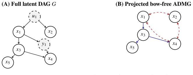
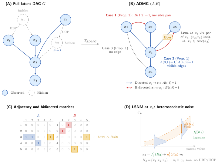
read the original abstract

We study causal discovery from observational data when some variables are hidden and the data-generating process follows a location-scale noise model (LSNM). Existing methods that handle hidden confounders typically assume additive noise, but in practice, causes often modulate not just the mean but also the variance of their effects. We prove that acyclic directed mixed graphs (ADMGs) satisfying a bow-free condition are identifiable under LSNM with hidden variables, establishing the first identifiability result for causally insufficient models beyond noise additivity. We further provide sufficient conditions for identifying causal direction even when the bow-free assumption is violated. Our two-stage algorithm, LSNM-UV, is sound and complete, and experiments demonstrate improved performance over additive baselines on heteroscedastic data.

Editorial analysis

A structured set of objections, weighed in public.

Desk editor's note, referee report, simulated authors' rebuttal, and a circularity audit. Tearing a paper down is the easy half of reading it; the pith above is the substance, this is the friction.

Desk Editor's Note private letter to a colleague

The paper gives the first identifiability theorem for bow-free ADMGs under location-scale noise with hidden variables.

read the letter

The main takeaway is that this work proves identifiability for acyclic directed mixed graphs under location-scale noise models even when some variables are hidden. That moves beyond the additive noise restriction that has dominated most prior results with latent confounders.

They establish that bow-free ADMGs are identifiable in this setting and supply extra conditions that recover direction even if the bow-free property fails. The two-stage algorithm LSNM-UV is presented as sound and complete, and the experiments indicate gains over additive baselines precisely when heteroscedasticity is present.

The extension itself is useful because many real processes let a cause change both the mean and the spread of an effect. The modeling choice is stated clearly and the graphical restriction is explicit, so the scope of the claim is easy to understand.

The soft spot is that the abstract supplies no derivation steps or error bounds, which makes it impossible to judge how tight the argument is or whether it introduces unstated restrictions. The experimental section is summarized without numbers or setup details, so the practical improvement is hard to weigh. Those gaps are typical for an initial submission but still need checking.

This is for researchers who build causal discovery methods that must handle both latent variables and non-additive noise. A reader focused on identifiability theorems would find the result worth examining.

It deserves peer review. The claim is specific, the motivation is reasonable, and the central argument does not appear to contain internal contradictions from what is shown.

Referee Report

0 major / 2 minor

Summary. The paper claims to prove that acyclic directed mixed graphs (ADMGs) satisfying a bow-free condition are identifiable under location-scale noise models (LSNM) with hidden variables. It establishes this as the first identifiability result for causally insufficient models beyond additive noise, provides sufficient conditions for identifying causal direction even when the bow-free assumption is violated, introduces the two-stage LSNM-UV algorithm claimed to be sound and complete, and reports experiments showing improved performance over additive baselines on heteroscedastic data.

Significance. If the identifiability theorem and soundness/completeness of LSNM-UV hold, the result would meaningfully extend causal discovery beyond additive noise assumptions to location-scale models that capture variance modulation, while accommodating hidden variables via ADMGs. This addresses a practical limitation of existing methods and could enable more realistic modeling of heteroscedastic causal effects.

minor comments (2)

The abstract asserts a proof of identifiability and that the algorithm is sound and complete but supplies no derivation steps, key lemmas, or error analysis; the central claim therefore cannot be evaluated from the provided information.
Experimental details (datasets, metrics, baselines, and quantitative results) are referenced but not described in the abstract, limiting assessment of the performance claims.

Simulated Author's Rebuttal

0 responses · 0 unresolved

We thank the referee for their review and for recognizing the potential significance of extending causal discovery to location-scale noise models with hidden variables. The report notes an 'uncertain' recommendation but provides no specific major comments for us to address point by point. We remain available to provide additional clarifications or revisions if the editor or referee identifies particular concerns.

Circularity Check

0 steps flagged

No significant circularity detected

full rationale

The paper advances a theoretical identifiability theorem for bow-free ADMGs under the location-scale noise model with hidden variables. The derivation is presented as a direct proof from the stated graphical and distributional assumptions (LSNM rather than additive noise), without any reduction of the central claim to fitted parameters, self-referential definitions, or load-bearing self-citations whose validity depends on the present work. The bow-free condition and LSNM scope are explicitly declared as the enabling restrictions, and the result is framed as extending prior additive-noise results rather than re-deriving them by construction. This is the most common honest outcome for a pure identifiability paper whose assumptions are stated up front.

Axiom & Free-Parameter Ledger

0 free parameters · 2 axioms · 0 invented entities

The central claim rests on the modeling assumption that the data follows a location-scale noise model and on the bow-free restriction on the ADMG; no free parameters or new entities appear in the abstract.

axioms (2)

domain assumption Observed data are generated by an acyclic directed mixed graph under a location-scale noise model.
Core modeling assumption required for the stated identifiability.
domain assumption The graph satisfies the bow-free condition.
Explicitly required for the main identifiability theorem.

pith-pipeline@v0.9.1-grok · 5661 in / 1167 out tokens · 25385 ms · 2026-06-27T19:14:37.587002+00:00 · methodology

discussion (0)

Reference graph

Works this paper leans on

26 extracted references · 1 canonical work pages

[1]

Causal reasoning in the presence of latent confounders via neural ADMG learning

Matthew Ashman, Chao Ma, Agrin Hilmkil, Joel Jennings, and Cheng Zhang. Causal reasoning in the presence of latent confounders via neural ADMG learning. InThe 11th International Conference on Learning Representations (ICLR), 2023. 10

2023
[2]

CAM: Causal additive models, high-dimensional order search and penalized regression.The Annals of Statistics, 42(6):2526–2556, 2014

Peter Bühlmann, Jonas Peters, and Jan Ernest. CAM: Causal additive models, high-dimensional order search and penalized regression.The Annals of Statistics, 42(6):2526–2556, 2014

2014
[3]

Hoyer, Shohei Shimizu, Antti J

Patrik O. Hoyer, Shohei Shimizu, Antti J. Kerminen, and Markus Palviainen. Causal discovery of linear acyclic models with arbitrary distributions. InProceedings of the 24th Conference on Uncertainty in Artificial Intelligence (UAI), pages 282–289, 2008

2008
[4]

Hoyer, Dominik Janzing, Joris M

Patrik O. Hoyer, Dominik Janzing, Joris M. Mooij, Jonas Peters, and Bernhard Schölkopf. Nonlinear causal discovery with additive noise models. InAdvances in Neural Information Processing Systems 21 (NeurIPS), pages 689–696, 2009

2009
[5]

Vogt, Bernhard Schölkopf, Peter Bühlmann, and Alexander Marx

Alexander Immer, Christoph Schultheiss, Julia E. Vogt, Bernhard Schölkopf, Peter Bühlmann, and Alexander Marx. On the identifiability and estimation of causal location-scale noise models. InProceedings of the 40th International Conference on Machine Learning (ICML), volume 202 ofPMLR, pages 14316–14332, 2023

2023
[6]

A skewness-based criterion for addressing heteroscedastic noise in causal discovery

Yingyu Lin, Yuxing Huang, Wenqin Liu, Haoran Deng, Ignavier Ng, Kun Zhang, Mingming Gong, Yian Ma, and Biwei Huang. A skewness-based criterion for addressing heteroscedastic noise in causal discovery. InThe 13th International Conference on Learning Representations (ICLR), 2025

2025
[7]

Causaladditivemodelswithunobservedvariables

TakashiNicholasMaedaandShoheiShimizu. Causaladditivemodelswithunobservedvariables. InProceedings of the 37th Conference on Uncertainty in Artificial Intelligence (UAI), volume 161 ofPMLR, pages 97–106, 2021

2021
[8]

Cambridge University Press, 2nd edition, 2009

Judea Pearl.Causality: Models, Reasoning, and Inference. Cambridge University Press, 2nd edition, 2009

2009
[9]

Mooij, Dominik Janzing, and Bernhard Schölkopf

Jonas Peters, Joris M. Mooij, Dominik Janzing, and Bernhard Schölkopf. Identifiability of causal graphs using functional models. InProceedings of the 27th Conference on Uncertainty in Artificial Intelligence (UAI), pages 589–598, 2011

2011
[10]

Mooij, Dominik Janzing, and Bernhard Schölkopf

Jonas Peters, Joris M. Mooij, Dominik Janzing, and Bernhard Schölkopf. Causal discovery with continuous additive noise models.Journal of Machine Learning Research, 15(58):2009–2053, 2014

2009
[11]

Causal additive models with unobserved causal paths and backdoor paths

Thong Pham, Takashi Nicholas Maeda, and Shohei Shimizu. Causal additive models with unobserved causal paths and backdoor paths. InThe 29th International Conference on Artificial Intelligence and Statistics, 2026

2026
[12]

Markov Properties for Acyclic Directed Mixed Graphs , volume=

Thomas Richardson. Markov properties for acyclic directed mixed graphs.Scandinavian Journal of Statistics, 30(1):145–157, 2003. doi: 10.1111/1467-9469.00323

work page doi:10.1111/1467-9469.00323 2003
[13]

AncestralgraphMarkovmodels.TheAnnalsofStatistics, 30(4):962–1030, 2002

ThomasRichardsonandPeterSpirtes. AncestralgraphMarkovmodels.TheAnnalsofStatistics, 30(4):962–1030, 2002

2002
[14]

Hoyer, Aapo Hyvärinen, and Antti Kerminen

Shohei Shimizu, Patrik O. Hoyer, Aapo Hyvärinen, and Antti Kerminen. A linear non-Gaussian acyclic model for causal discovery.Journal of Machine Learning Research, 7:2003–2030, 2006

2003
[15]

Glymour, and Richard Scheines.Causation, Prediction, and Search

Peter Spirtes, Clark N. Glymour, and Richard Scheines.Causation, Prediction, and Search. MIT Press, Cambridge, MA, 2nd edition, 2000

2000
[16]

Cause-effect inference in location-scale noise models: Maximum likelihood vs

Xiangyu Sun and Oliver Schulte. Cause-effect inference in location-scale noise models: Maximum likelihood vs. independence testing. InAdvances in Neural Information Processing Systems 36 (NeurIPS), 2023

2023
[17]

Samuel Wang and Mathias Drton

Y. Samuel Wang and Mathias Drton. Causal discovery with unobserved confounding and non-Gaussian data.Journal of Machine Learning Research, 24(271):1–61, 2023. 11

2023
[18]

Effective causal discovery under identifiable heteroscedastic noise model

Naiyu Yin, Tian Gao, Yue Yu, and Qiang Ji. Effective causal discovery under identifiable heteroscedastic noise model. InProceedings of the 38th AAAI Conference on Artificial Intelligence, volume 38, 2024

2024
[19]

On the completeness of orientation rules for causal discovery in the presence of latent confounders and selection bias.Artificial Intelligence, 172(16–17):1873–1896, 2008

Jiji Zhang. On the completeness of orientation rules for causal discovery in the presence of latent confounders and selection bias.Artificial Intelligence, 172(16–17):1873–1896, 2008

2008
[20]

visible edge,

Kun Zhang and Aapo Hyvärinen. On the identifiability of the post-nonlinear causal model. InProceedings of the 25th Conference on Uncertainty in Artificial Intelligence (UAI), pages 647–655, 2009. A Technical appendices and supplementary material A.1 Theoretical proofs Notation.In the main text, the regression functionℎ(𝑖, 𝑆) uses a single exclusion set𝑆 f...

2009
[21]

, 𝑚 , the pair (𝑥𝑖, 𝑥𝑘𝑞 ) is invisible (Definition A.3): ∀ℎ 1, ℎ2 ∈ H : ℎ1(𝑖,{𝑖}) ̸ ⊥ ⊥ℎ2(𝑘 𝑞,{𝑘 𝑞 })

For each 𝑞=1, . . . , 𝑚 , the pair (𝑥𝑖, 𝑥𝑘𝑞 ) is invisible (Definition A.3): ∀ℎ 1, ℎ2 ∈ H : ℎ1(𝑖,{𝑖}) ̸ ⊥ ⊥ℎ2(𝑘 𝑞,{𝑘 𝑞 }). Under Assumptions 1 and 2, suppose further that for each𝑞=1, . . . , 𝑚the following holds: ∀ℎ 1, ℎ2 ∈ H:ℎ 1(𝑖,{𝑖, 𝑘 𝑞 }) ̸ ⊥ ⊥ℎ 2 (𝑗,{𝑗, 𝑘 𝑞 }).(25) Then each𝑥𝑘𝑞 is an ancestor of𝑥𝑖. Proof. Fix any𝑞∈ {1, . . . , 𝑚} . We prove the cont...
[22]

Select a pair(𝑥 𝑎, 𝑥𝑏) of observed variables that have no direct edge between them in either direction
[23]

The node𝑢𝑘 is a root (no parents of its own)

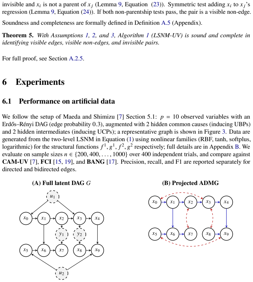
Add directed edges𝑢𝑘 →𝑥 𝑎 and𝑢 𝑘 →𝑥 𝑏. The node𝑢𝑘 is a root (no parents of its own). When 𝑢𝑘 ismarginalisedout,theprojectedADMGacquiresthebidirectededge 𝑥𝑎 ↔𝑥 𝑏,representing an Unobserved Backdoor Path (UBP). Because(𝑥 𝑎, 𝑥𝑏) was chosen to have no direct edge, the bow-free condition is satisfied for this pair. Hidden intermediates (UCPs).For each of the𝑛i...
[24]

2.Removethe direct edge𝑥 𝑗 →𝑥 𝑖

Select an existing direct observed edge𝑥𝑗 →𝑥 𝑖. 2.Removethe direct edge𝑥 𝑗 →𝑥 𝑖
[25]

When 𝑦𝑘 ismarginalisedout,theprojectedADMGacquiresthebidirectededge 𝑥 𝑗 ↔𝑥 𝑖,representing an Unobserved Causal Path (UCP)

Add𝑥 𝑗 →𝑦 𝑘 and𝑦 𝑘 →𝑥 𝑖. When 𝑦𝑘 ismarginalisedout,theprojectedADMGacquiresthebidirectededge 𝑥 𝑗 ↔𝑥 𝑖,representing an Unobserved Causal Path (UCP). Removing the direct edge ensures bow-freeness. Step 2: Data generation All variables are generated in topological order of the full latent DAG, so that every parent of𝑣 𝑖 has already been assigned values when𝑣...
[26]

• FCI[ 15, 19]

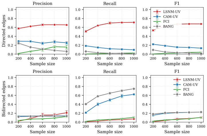
Output parsing identical to LSNM-UV. • FCI[ 15, 19]. From the causal-learn package (v0.1.4.5) with Fisher-𝑧 test at 𝛼=0.01 . We extract onlydefiniteedges (no circle marks): directed𝑥 𝑗 →𝑥 𝑖 when 𝐺[𝑗, 𝑖]=−1 and 𝐺[𝑖, 𝑗]=1; bidirected𝑥 𝑖 ↔𝑥 𝑗 when𝐺[𝑖, 𝑗]=𝐺[𝑗, 𝑖]=1. • BANG[17]. Sourcefrom https://github.com/ysamwang/ngBap,calledvia rpy2(v3.5.11, Rv4.3.1). Run...

[1] [1]

Causal reasoning in the presence of latent confounders via neural ADMG learning

Matthew Ashman, Chao Ma, Agrin Hilmkil, Joel Jennings, and Cheng Zhang. Causal reasoning in the presence of latent confounders via neural ADMG learning. InThe 11th International Conference on Learning Representations (ICLR), 2023. 10

2023

[2] [2]

CAM: Causal additive models, high-dimensional order search and penalized regression.The Annals of Statistics, 42(6):2526–2556, 2014

Peter Bühlmann, Jonas Peters, and Jan Ernest. CAM: Causal additive models, high-dimensional order search and penalized regression.The Annals of Statistics, 42(6):2526–2556, 2014

2014

[3] [3]

Hoyer, Shohei Shimizu, Antti J

Patrik O. Hoyer, Shohei Shimizu, Antti J. Kerminen, and Markus Palviainen. Causal discovery of linear acyclic models with arbitrary distributions. InProceedings of the 24th Conference on Uncertainty in Artificial Intelligence (UAI), pages 282–289, 2008

2008

[4] [4]

Hoyer, Dominik Janzing, Joris M

Patrik O. Hoyer, Dominik Janzing, Joris M. Mooij, Jonas Peters, and Bernhard Schölkopf. Nonlinear causal discovery with additive noise models. InAdvances in Neural Information Processing Systems 21 (NeurIPS), pages 689–696, 2009

2009

[5] [5]

Vogt, Bernhard Schölkopf, Peter Bühlmann, and Alexander Marx

Alexander Immer, Christoph Schultheiss, Julia E. Vogt, Bernhard Schölkopf, Peter Bühlmann, and Alexander Marx. On the identifiability and estimation of causal location-scale noise models. InProceedings of the 40th International Conference on Machine Learning (ICML), volume 202 ofPMLR, pages 14316–14332, 2023

2023

[6] [6]

A skewness-based criterion for addressing heteroscedastic noise in causal discovery

Yingyu Lin, Yuxing Huang, Wenqin Liu, Haoran Deng, Ignavier Ng, Kun Zhang, Mingming Gong, Yian Ma, and Biwei Huang. A skewness-based criterion for addressing heteroscedastic noise in causal discovery. InThe 13th International Conference on Learning Representations (ICLR), 2025

2025

[7] [7]

Causaladditivemodelswithunobservedvariables

TakashiNicholasMaedaandShoheiShimizu. Causaladditivemodelswithunobservedvariables. InProceedings of the 37th Conference on Uncertainty in Artificial Intelligence (UAI), volume 161 ofPMLR, pages 97–106, 2021

2021

[8] [8]

Cambridge University Press, 2nd edition, 2009

Judea Pearl.Causality: Models, Reasoning, and Inference. Cambridge University Press, 2nd edition, 2009

2009

[9] [9]

Mooij, Dominik Janzing, and Bernhard Schölkopf

Jonas Peters, Joris M. Mooij, Dominik Janzing, and Bernhard Schölkopf. Identifiability of causal graphs using functional models. InProceedings of the 27th Conference on Uncertainty in Artificial Intelligence (UAI), pages 589–598, 2011

2011

[10] [10]

Mooij, Dominik Janzing, and Bernhard Schölkopf

Jonas Peters, Joris M. Mooij, Dominik Janzing, and Bernhard Schölkopf. Causal discovery with continuous additive noise models.Journal of Machine Learning Research, 15(58):2009–2053, 2014

2009

[11] [11]

Causal additive models with unobserved causal paths and backdoor paths

Thong Pham, Takashi Nicholas Maeda, and Shohei Shimizu. Causal additive models with unobserved causal paths and backdoor paths. InThe 29th International Conference on Artificial Intelligence and Statistics, 2026

2026

[12] [12]

Markov Properties for Acyclic Directed Mixed Graphs , volume=

Thomas Richardson. Markov properties for acyclic directed mixed graphs.Scandinavian Journal of Statistics, 30(1):145–157, 2003. doi: 10.1111/1467-9469.00323

work page doi:10.1111/1467-9469.00323 2003

[13] [13]

AncestralgraphMarkovmodels.TheAnnalsofStatistics, 30(4):962–1030, 2002

ThomasRichardsonandPeterSpirtes. AncestralgraphMarkovmodels.TheAnnalsofStatistics, 30(4):962–1030, 2002

2002

[14] [14]

Hoyer, Aapo Hyvärinen, and Antti Kerminen

Shohei Shimizu, Patrik O. Hoyer, Aapo Hyvärinen, and Antti Kerminen. A linear non-Gaussian acyclic model for causal discovery.Journal of Machine Learning Research, 7:2003–2030, 2006

2003

[15] [15]

Glymour, and Richard Scheines.Causation, Prediction, and Search

Peter Spirtes, Clark N. Glymour, and Richard Scheines.Causation, Prediction, and Search. MIT Press, Cambridge, MA, 2nd edition, 2000

2000

[16] [16]

Cause-effect inference in location-scale noise models: Maximum likelihood vs

Xiangyu Sun and Oliver Schulte. Cause-effect inference in location-scale noise models: Maximum likelihood vs. independence testing. InAdvances in Neural Information Processing Systems 36 (NeurIPS), 2023

2023

[17] [17]

Samuel Wang and Mathias Drton

Y. Samuel Wang and Mathias Drton. Causal discovery with unobserved confounding and non-Gaussian data.Journal of Machine Learning Research, 24(271):1–61, 2023. 11

2023

[18] [18]

Effective causal discovery under identifiable heteroscedastic noise model

Naiyu Yin, Tian Gao, Yue Yu, and Qiang Ji. Effective causal discovery under identifiable heteroscedastic noise model. InProceedings of the 38th AAAI Conference on Artificial Intelligence, volume 38, 2024

2024

[19] [19]

On the completeness of orientation rules for causal discovery in the presence of latent confounders and selection bias.Artificial Intelligence, 172(16–17):1873–1896, 2008

Jiji Zhang. On the completeness of orientation rules for causal discovery in the presence of latent confounders and selection bias.Artificial Intelligence, 172(16–17):1873–1896, 2008

2008

[20] [20]

visible edge,

Kun Zhang and Aapo Hyvärinen. On the identifiability of the post-nonlinear causal model. InProceedings of the 25th Conference on Uncertainty in Artificial Intelligence (UAI), pages 647–655, 2009. A Technical appendices and supplementary material A.1 Theoretical proofs Notation.In the main text, the regression functionℎ(𝑖, 𝑆) uses a single exclusion set𝑆 f...

2009

[21] [21]

, 𝑚 , the pair (𝑥𝑖, 𝑥𝑘𝑞 ) is invisible (Definition A.3): ∀ℎ 1, ℎ2 ∈ H : ℎ1(𝑖,{𝑖}) ̸ ⊥ ⊥ℎ2(𝑘 𝑞,{𝑘 𝑞 })

For each 𝑞=1, . . . , 𝑚 , the pair (𝑥𝑖, 𝑥𝑘𝑞 ) is invisible (Definition A.3): ∀ℎ 1, ℎ2 ∈ H : ℎ1(𝑖,{𝑖}) ̸ ⊥ ⊥ℎ2(𝑘 𝑞,{𝑘 𝑞 }). Under Assumptions 1 and 2, suppose further that for each𝑞=1, . . . , 𝑚the following holds: ∀ℎ 1, ℎ2 ∈ H:ℎ 1(𝑖,{𝑖, 𝑘 𝑞 }) ̸ ⊥ ⊥ℎ 2 (𝑗,{𝑗, 𝑘 𝑞 }).(25) Then each𝑥𝑘𝑞 is an ancestor of𝑥𝑖. Proof. Fix any𝑞∈ {1, . . . , 𝑚} . We prove the cont...

[22] [22]

Select a pair(𝑥 𝑎, 𝑥𝑏) of observed variables that have no direct edge between them in either direction

[23] [23]

The node𝑢𝑘 is a root (no parents of its own)

Add directed edges𝑢𝑘 →𝑥 𝑎 and𝑢 𝑘 →𝑥 𝑏. The node𝑢𝑘 is a root (no parents of its own). When 𝑢𝑘 ismarginalisedout,theprojectedADMGacquiresthebidirectededge 𝑥𝑎 ↔𝑥 𝑏,representing an Unobserved Backdoor Path (UBP). Because(𝑥 𝑎, 𝑥𝑏) was chosen to have no direct edge, the bow-free condition is satisfied for this pair. Hidden intermediates (UCPs).For each of the𝑛i...

[24] [24]

2.Removethe direct edge𝑥 𝑗 →𝑥 𝑖

Select an existing direct observed edge𝑥𝑗 →𝑥 𝑖. 2.Removethe direct edge𝑥 𝑗 →𝑥 𝑖

[25] [25]

When 𝑦𝑘 ismarginalisedout,theprojectedADMGacquiresthebidirectededge 𝑥 𝑗 ↔𝑥 𝑖,representing an Unobserved Causal Path (UCP)

Add𝑥 𝑗 →𝑦 𝑘 and𝑦 𝑘 →𝑥 𝑖. When 𝑦𝑘 ismarginalisedout,theprojectedADMGacquiresthebidirectededge 𝑥 𝑗 ↔𝑥 𝑖,representing an Unobserved Causal Path (UCP). Removing the direct edge ensures bow-freeness. Step 2: Data generation All variables are generated in topological order of the full latent DAG, so that every parent of𝑣 𝑖 has already been assigned values when𝑣...

[26] [26]

• FCI[ 15, 19]

Output parsing identical to LSNM-UV. • FCI[ 15, 19]. From the causal-learn package (v0.1.4.5) with Fisher-𝑧 test at 𝛼=0.01 . We extract onlydefiniteedges (no circle marks): directed𝑥 𝑗 →𝑥 𝑖 when 𝐺[𝑗, 𝑖]=−1 and 𝐺[𝑖, 𝑗]=1; bidirected𝑥 𝑖 ↔𝑥 𝑗 when𝐺[𝑖, 𝑗]=𝐺[𝑗, 𝑖]=1. • BANG[17]. Sourcefrom https://github.com/ysamwang/ngBap,calledvia rpy2(v3.5.11, Rv4.3.1). Run...