AESTRA II: Generative Spectral Modeling of the Sun as a Star for Precise Radial Velocities
Pith reviewed 2026-06-27 05:29 UTC · model grok-4.3
The pith
Generative spectral model recovers 238 of 500 injected planets, including 13 below 0.3 m/s, versus 9 for standard methods.
A machine-rendered reading of the paper's core claim, the machinery that carries it, and where it could break.
Core claim
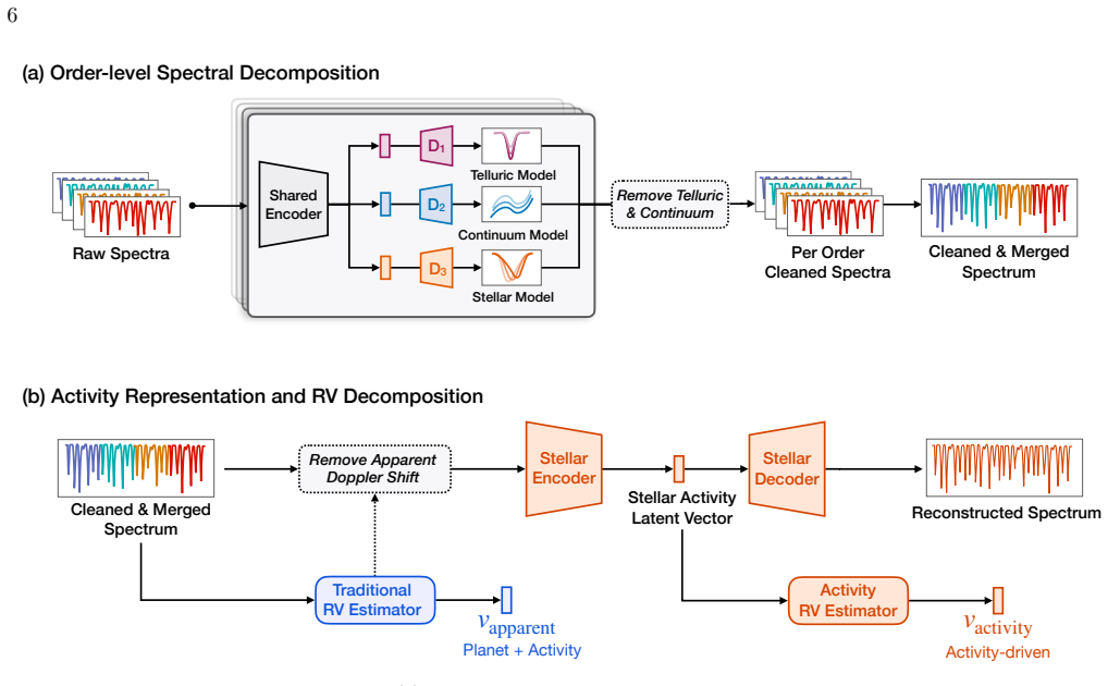
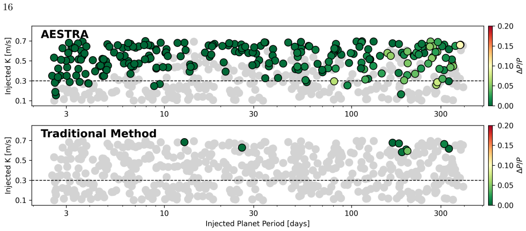
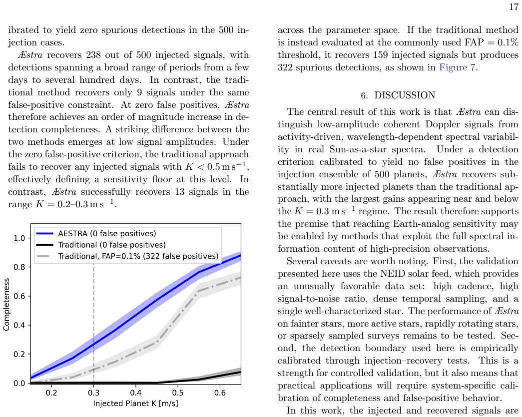
AESTRA empirically decomposes the spectra into stellar line-shape variability, micro-telluric absorption, and continuum variability without external templates. After removing the learned telluric and continuum components, it trains a low-dimensional representation of the spectrum to infer activity-driven apparent RVs jointly with candidate Doppler signals. In 500 single-planet injection-recovery tests, AESTRA recovers 238 injected planets including 13 with K < 0.3 m s^{-1}, whereas traditional CCF-based activity-indicator detrending recovers 9 planets and none below K = 0.5 m s^{-1}.
What carries the argument
AESTRA's empirical generative decomposition into line-shape variability, micro-telluric absorption, and continuum variability, followed by a low-dimensional spectral representation for joint RV inference.
If this is right
- Planets with semi-amplitudes between 0.1 and 0.5 m/s become detectable at the same false-positive rate where traditional methods find none.
- Activity and planetary signals can be inferred together from one low-dimensional model without separate activity indicators.
- The zero-spurious-detection calibration allows higher true-positive rates while preserving search purity.
- Reliance on external stellar or atmospheric templates is eliminated for this class of modeling.
- The method scales to longer time series by continuing to learn components directly from the data.
Where Pith is reading between the lines
- Application to other stars observed with the same instrument could extend the recovery gain beyond the Sun.
- The same decomposition might be tested on multi-planet systems to check whether multiple signals remain separable.
- Combining the low-dimensional representation with existing activity proxies could further lower the detection threshold.
- Archival spectra from other EPRV spectrographs offer a direct test of whether the performance gain transfers.
Load-bearing premise
The learned decomposition into activity, telluric, and continuum components leaves genuine planetary Doppler signals untouched.
What would settle it
A controlled test in which injected planetary signals below 0.3 m/s are systematically attenuated or removed after the decomposition step would falsify the recovery advantage.
Figures

read the original abstract
The detection of Earth analogs with extreme-precision radial velocities (EPRVs) is limited by spectral variability from stellar activity, telluric absorption, and instrumental systematics. We apply AESTRA, a generative spectrum modeling framework, to NEID Sun-as-a-star observations. AESTRA empirically decomposes the spectra into stellar line-shape variability, micro-telluric absorption, and continuum variability without external atmospheric or stellar templates. After removing the learned telluric and continuum components, we train a low-dimensional representation of the spectrum to infer activity-driven apparent RVs jointly with candidate Doppler signals. We evaluate the method with 500 single-planet injection-recovery tests spanning periods of 2.5 to 400 days and semi-amplitudes of K = 0.1 to 0.7 m s^-1, calibrating the detection criterion to yield zero spurious detections. At this matched confidence level, AESTRA recovers 238 injected planets, including 13 with K < 0.3 m s^-1, whereas traditional CCF-based activity-indicator detrending recovers 9 planets and none below K = 0.5 m s^-1.
Editorial analysis
A structured set of objections, weighed in public.
Referee Report
Summary. The paper presents AESTRA II, a generative framework that empirically decomposes NEID Sun-as-a-star spectra into stellar line-shape variability, micro-telluric absorption, and continuum variability without external templates. After removing the telluric and continuum components, a low-dimensional representation is trained on the residuals to jointly infer activity-driven apparent RVs and candidate planetary Doppler signals. Evaluated via 500 single-planet injection-recovery tests (periods 2.5–400 days, K = 0.1–0.7 m s⁻¹) with a detection threshold calibrated to zero false positives, the method recovers 238 injected planets (including 13 with K < 0.3 m s⁻¹), compared to 9 planets (none below K = 0.5 m s⁻¹) using traditional CCF-based activity-indicator detrending.
Significance. If the central performance claims hold after addressing the training-data circularity, the approach could meaningfully advance EPRV sensitivity by reducing the impact of stellar activity and tellurics on low-amplitude signals, offering a data-driven alternative to template-based methods for Sun-like stars.
major comments (3)
- [Abstract / generative decomposition description] Abstract and method description: The generative decomposition into line-shape, micro-telluric, and continuum components is trained on the same NEID spectra that contain the 500 injected planetary signals. Any correlation between the injected Doppler shifts and the learned components risks partial absorption of planetary signals into the removed terms or the subsequent activity model, directly undermining the reported recovery counts (238 planets, 13 with K < 0.3 m s⁻¹). An explicit test (e.g., training on uninjected data or measuring recovered K versus injected K in the absence of activity) is required to validate the weakest assumption.
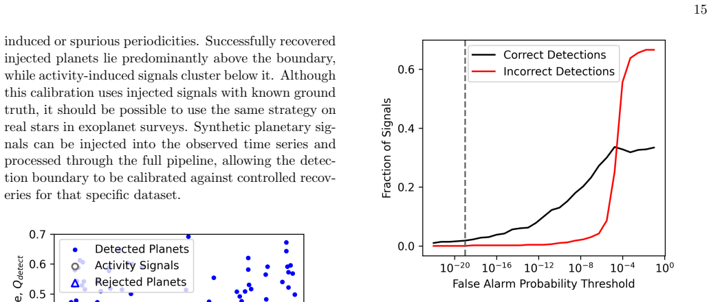
- [Injection-recovery tests] Injection-recovery section: The detection criterion is calibrated to produce zero spurious detections, yet the manuscript provides no derivation of the threshold, error propagation details, or data exclusion rules. Without these, the quantitative superiority over CCF methods cannot be independently verified from the 500 tests.
- [Low-dimensional representation and joint inference] Low-dimensional representation training: The activity-driven RV inference is performed jointly with candidate signals on residuals from the same dataset used to learn the decomposition. This creates a circularity burden where the model may misattribute or attenuate genuine Doppler signals as activity variability, and no cross-validation or hold-out test separating training spectra from injected signals is described.
minor comments (2)
- [Method] Notation for the low-dimensional basis and activity indicators should be defined explicitly with equations rather than descriptive text only.
- [Figures] Figure captions for the injection-recovery results should include the exact number of tests per K bin and the precise false-positive calibration procedure.
Simulated Author's Rebuttal
We thank the referee for their thorough review and for highlighting important concerns about potential circularity and methodological transparency. We address each major comment below. Where the comments identify gaps that require additional validation or documentation, we will revise the manuscript accordingly.
read point-by-point responses
-
Referee: [Abstract / generative decomposition description] Abstract and method description: The generative decomposition into line-shape, micro-telluric, and continuum components is trained on the same NEID spectra that contain the 500 injected planetary signals. Any correlation between the injected Doppler shifts and the learned components risks partial absorption of planetary signals into the removed terms or the subsequent activity model, directly undermining the reported recovery counts (238 planets, 13 with K < 0.3 m s⁻¹). An explicit test (e.g., training on uninjected data or measuring recovered K versus injected K in the absence of activity) is required to validate the weakest assumption.
Authors: We agree that this is a substantive concern. The decomposition is intended to isolate line-shape variability, micro-tellurics, and continuum effects, with planetary Doppler shifts handled in the subsequent low-dimensional RV inference step. However, because the decomposition was trained on the injected dataset, we cannot rule out partial absorption without further testing. We will add an explicit validation test training the decomposition exclusively on uninjected spectra and then applying the full pipeline to the injected set, reporting the resulting recovery statistics in the revised manuscript. revision: yes
-
Referee: [Injection-recovery tests] Injection-recovery section: The detection criterion is calibrated to produce zero spurious detections, yet the manuscript provides no derivation of the threshold, error propagation details, or data exclusion rules. Without these, the quantitative superiority over CCF methods cannot be independently verified from the 500 tests.
Authors: We accept this criticism. The current text states only that the threshold was calibrated to zero false positives but does not supply the derivation, error propagation, or exclusion criteria. In the revised manuscript we will include a dedicated subsection detailing the threshold derivation, the statistical procedure used to ensure zero spurious detections, the error propagation, and any data exclusion rules applied to the 500 tests. revision: yes
-
Referee: [Low-dimensional representation and joint inference] Low-dimensional representation training: The activity-driven RV inference is performed jointly with candidate signals on residuals from the same dataset used to learn the decomposition. This creates a circularity burden where the model may misattribute or attenuate genuine Doppler signals as activity variability, and no cross-validation or hold-out test separating training spectra from injected signals is described.
Authors: This point overlaps with the first comment. The joint inference occurs after the telluric/continuum removal step, but the low-dimensional representation is still learned from the same spectra. We will introduce a cross-validation or hold-out protocol that separates the spectra used to train the low-dimensional activity model from those used in the injection-recovery tests and will report the outcome of this test in the revision. revision: yes
Circularity Check
Low-dimensional representation trained on spectra containing injected signals, then used to recover those signals
specific steps
-
fitted input called prediction
[Abstract]
"After removing the learned telluric and continuum components, we train a low-dimensional representation of the spectrum to infer activity-driven apparent RVs jointly with candidate Doppler signals. We evaluate the method with 500 single-planet injection-recovery tests spanning periods of 2.5 to 400 days and semi-amplitudes of K = 0.1 to 0.7 m s^-1, calibrating the detection criterion to yield zero spurious detections. At this matched confidence level, AESTRA recovers 238 injected planets, including 13 with K < 0.3 m s^-1"
The low-dimensional representation is trained on the identical spectra containing the 500 injected planetary signals. The inference of activity RVs jointly with candidate Doppler signals, followed by counting recoveries from those same data, reduces the 'recovery' counts to a fitted outcome on the training inputs rather than an out-of-sample prediction.
full rationale
The paper's evaluation uses injection-recovery tests on the same NEID spectra from which the generative decomposition and low-dimensional representation are learned. This setup means the reported recovery of 238 planets (including weak ones) occurs after fitting the activity model to data that already embeds the injected Doppler signals, creating moderate circularity in claiming superior separation without independent validation that signals are not partially absorbed. No self-citation chains or definitional reductions are evident from the abstract; the issue is specific to the fitted-input nature of the recovery metric.
Axiom & Free-Parameter Ledger
Reference graph
Works this paper leans on
-
[1]
2023, ARA&A, 61, 329, doi: 10.1146/annurev-astro-052920-103508
Aigrain, S., & Foreman-Mackey, D. 2023, ARA&A, 61, 329, doi: 10.1146/annurev-astro-052920-103508
-
[2]
2022, A&A, 666, A196, doi: 10.1051/0004-6361/202243629 Astropy Collaboration, Robitaille, T
Allart, R., Lovis, C., Faria, J., et al. 2022, A&A, 666, A196, doi: 10.1051/0004-6361/202243629 Astropy Collaboration, Robitaille, T. P., Tollerud, E. J., et al. 2013, A&A, 558, A33, doi: 10.1051/0004-6361/201322068 Astropy Collaboration, Price-Whelan, A. M., Sip˝ ocz, B. M., et al. 2018, AJ, 156, 123, doi: 10.3847/1538-3881/aabc4f Astropy Collaboration, ...
-
[3]
W., Foreman-Mackey, D., Montet, B
Bedell, M., Hogg, D. W., Foreman-Mackey, D., Montet, B. T., & Luger, R. 2019, AJ, 158, 164, doi: 10.3847/1538-3881/ab40a7
-
[4]
2014, A&A, 564, A46, doi: 10.1051/0004-6361/201322383
Bodichon, R. 2014, A&A, 564, A46, doi: 10.1051/0004-6361/201322383
-
[5]
Boisse, I., Bouchy, F., H´ ebrard, G., et al. 2011, A&A, 528, A4, doi: 10.1051/0004-6361/201014354
-
[6]
Clough, S. A., Shephard, M. W., Mlawer, E. J., et al. 2005, JQSRT, 91, 233, doi: 10.1016/j.jqsrt.2004.05.058 Collier Cameron, A., Ford, E. B., Shahaf, S., et al. 2021, MNRAS, 505, 1699, doi: 10.1093/mnras/stab1323
-
[7]
2020, A&A, 633, A76, doi: 10.1051/0004-6361/201936548
Lovis, C. 2020, A&A, 633, A76, doi: 10.1051/0004-6361/201936548
-
[8]
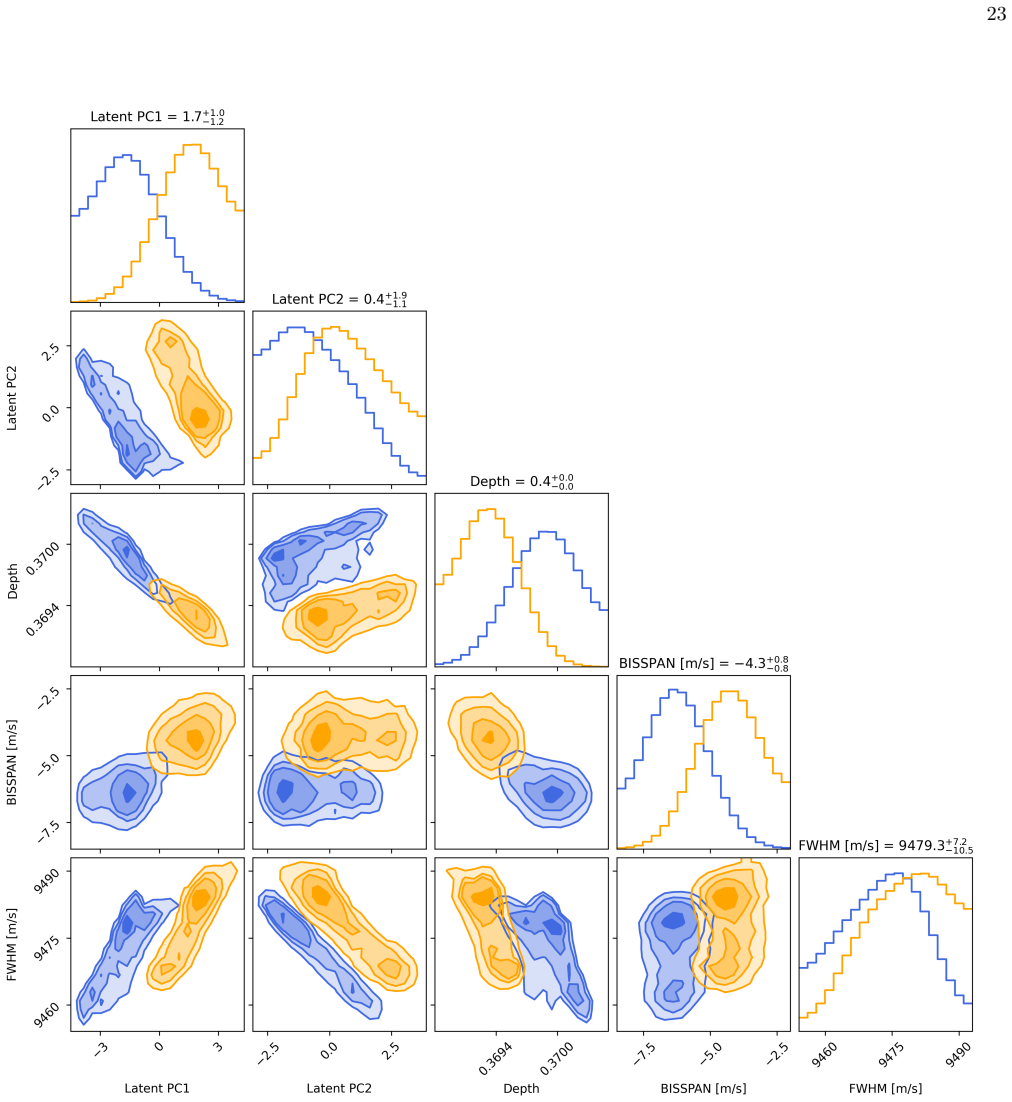
Cretignier, M., Dumusque, X., & Pepe, F. 2022, A&A, 659, A68, doi: 10.1051/0004-6361/202142435 23 Figure 10.Corner plot comparing the first two principal components of the learned stellar latent representation with tradi- tional CCF-based activity indicators, shown separately for the pre-fire (blue) and post-fire (orange) subsets. The two populations occu...
-
[9]
Cunha, D., Santos, N. C., Figueira, P., et al. 2014, A&A, 568, A35, doi: 10.1051/0004-6361/201423723 de Beurs, Z. L., Vanderburg, A., Shallue, C. J., et al. 2022, AJ, 164, 49, doi: 10.3847/1538-3881/ac738e
-
[10]
Dumusque, X., Boisse, I., & Santos, N. C. 2014, ApJ, 796, 132, doi: 10.1088/0004-637X/796/2/132
-
[11]
Monteiro, M. J. P. F. G. 2011, A&A, 525, A140, doi: 10.1051/0004-6361/201014097
-
[12]
Duncan, D. K., Vaughan, A. H., Wilson, O. C., et al. 1991, ApJS, 76, 383, doi: 10.1086/191572
-
[13]
Ford, E. B., Bender, C. F., Blake, C. H., et al. 2024, arXiv e-prints, arXiv:2408.13318, doi: 10.48550/arXiv.2408.13318
-
[14]
Gilbertson, C., Ford, E. B., Halverson, S., et al. 2024, arXiv e-prints, arXiv:2408.17289, doi: 10.48550/arXiv.2408.17289
-
[15]
D., Collier Cameron, A., Queloz, D., et al
Haywood, R. D., Collier Cameron, A., Queloz, D., et al. 2014, MNRAS, 443, 2517, doi: 10.1093/mnras/stu1320
-
[16]
A., Collier Cameron, A., Faria, J
John, A. A., Collier Cameron, A., Faria, J. P., et al. 2023, MNRAS, 525, 1687, doi: 10.1093/mnras/stad2381
-
[17]
2016, in Ground-based and airborne instrumentation for astronomy vi, Vol
Jurgenson, C., Fischer, D., McCracken, T., et al. 2016, in Ground-based and airborne instrumentation for astronomy vi, Vol. 9908, SPIE, 2051–2070
2016
-
[18]
1993, A&A, 271, 734
Lallement, R., Bertin, P., Chassefiere, E., & Scott, N. 1993, A&A, 271, 734
1993
-
[19]
Hodgkin, S. T. 2021, MNRAS, 502, 4392, doi: 10.1093/mnras/stab134
-
[20]
Liang, Y., Winn, J. N., & Melchior, P. 2024, AJ, 167, 23, doi: 10.3847/1538-3881/ad0e01
-
[21]
Lin, A. S. J., Monson, A., Mahadevan, S., et al. 2022, AJ, 163, 184, doi: 10.3847/1538-3881/ac5622
-
[22]
2023, The Astronomical Journal, 166, 74 NEID SpecSoft Team
Melchior, P., Liang, Y., Hahn, C., & Goulding, A. 2023, The Astronomical Journal, 166, 74 NEID SpecSoft Team. 2026, NEID RV Eras, https: //neid.ipac.caltech.edu/docs/NEID-DRP/rveras.html OpenAI. 2026, ChatGPT (2026 version), https://chatgpt.com/
2023
-
[23]
A., Cristiani, S., Lopez, R
Pepe, F. A., Cristiani, S., Lopez, R. R., et al. 2010, in Ground-based and Airborne Instrumentation for Astronomy III, Vol. 7735, SPIE, 209–217
2010
-
[24]
2015, MNRAS, 452, 2269, doi: 10.1093/mnras/stv1428
Roberts, S. 2015, MNRAS, 452, 2269, doi: 10.1093/mnras/stv1428
-
[25]
Robertson, P., Anderson, T., Stefansson, G., et al. 2019, Journal of Astronomical Telescopes, Instruments, and Systems, 5, 015003, doi: 10.1117/1.JATIS.5.1.015003
-
[26]
Schmidt, T. M., & Bouchy, F. 2024, MNRAS, 530, 1252, doi: 10.1093/mnras/stae920
-
[27]
2016, in Ground-based and airborne instrumentation for astronomy VI, Vol
Schwab, C., Rakich, A., Gong, Q., et al. 2016, in Ground-based and airborne instrumentation for astronomy VI, Vol. 9908, SPIE, 2220–2225
2016
-
[28]
2015, A&A, 576, A77, doi: 10.1051/0004-6361/201423932 St¨ urmer, J., Buchhave, L
Smette, A., Sana, H., Noll, S., et al. 2015, A&A, 576, A77, doi: 10.1051/0004-6361/201423932 St¨ urmer, J., Buchhave, L. A., Jessen, N. C., et al. 2024, in Society of Photo-Optical Instrumentation Engineers (SPIE) Conference Series, Vol. 13096, Ground-based and Airborne Instrumentation for Astronomy X, ed. J. J
-
[29]
Bryant, K. Motohara, & J. R. D. Vernet, 130968E, doi: 10.1117/12.3019107
-
[30]
J., Queloz, D., Baraffe, I., et al
Thompson, S. J., Queloz, D., Baraffe, I., et al. 2016, in Ground-based and Airborne Instrumentation for Astronomy VI, Vol. 9908, SPIE, 1949–1961
2016
-
[31]
2024, A&A, 687, A281, doi: 10.1051/0004-6361/202450022
Zhao, Y., Dumusque, X., Cretignier, M., et al. 2024, A&A, 687, A281, doi: 10.1051/0004-6361/202450022
discussion (0)
Sign in with ORCID, Apple, or X to comment. Anyone can read and Pith papers without signing in.