Disentangling the Distant Stellar Halo Using K-Giants in the DESI Year 3 Data
Pith reviewed 2026-06-26 20:35 UTC · model grok-4.3
The pith
The residual stellar halo shows similar bimodal metallicity distributions for both highly prograde and highly retrograde outer-halo K-giants.
A machine-rendered reading of the paper's core claim, the machinery that carries it, and where it could break.
Core claim
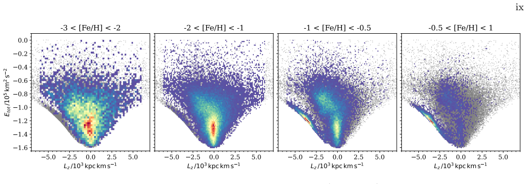
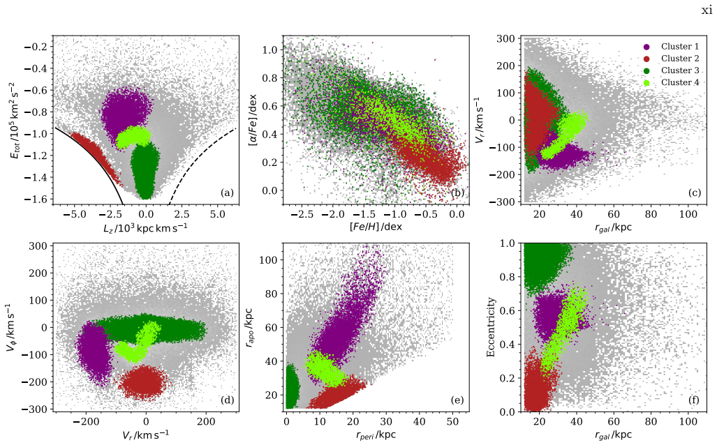
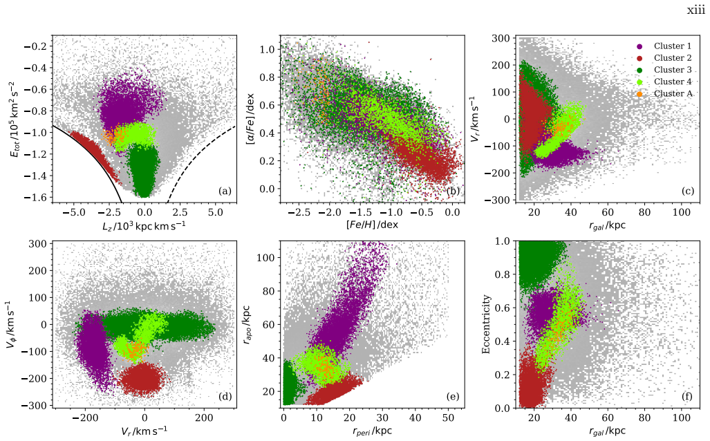
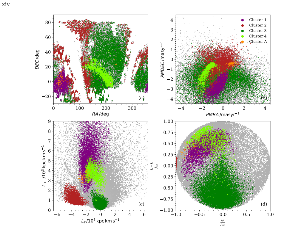
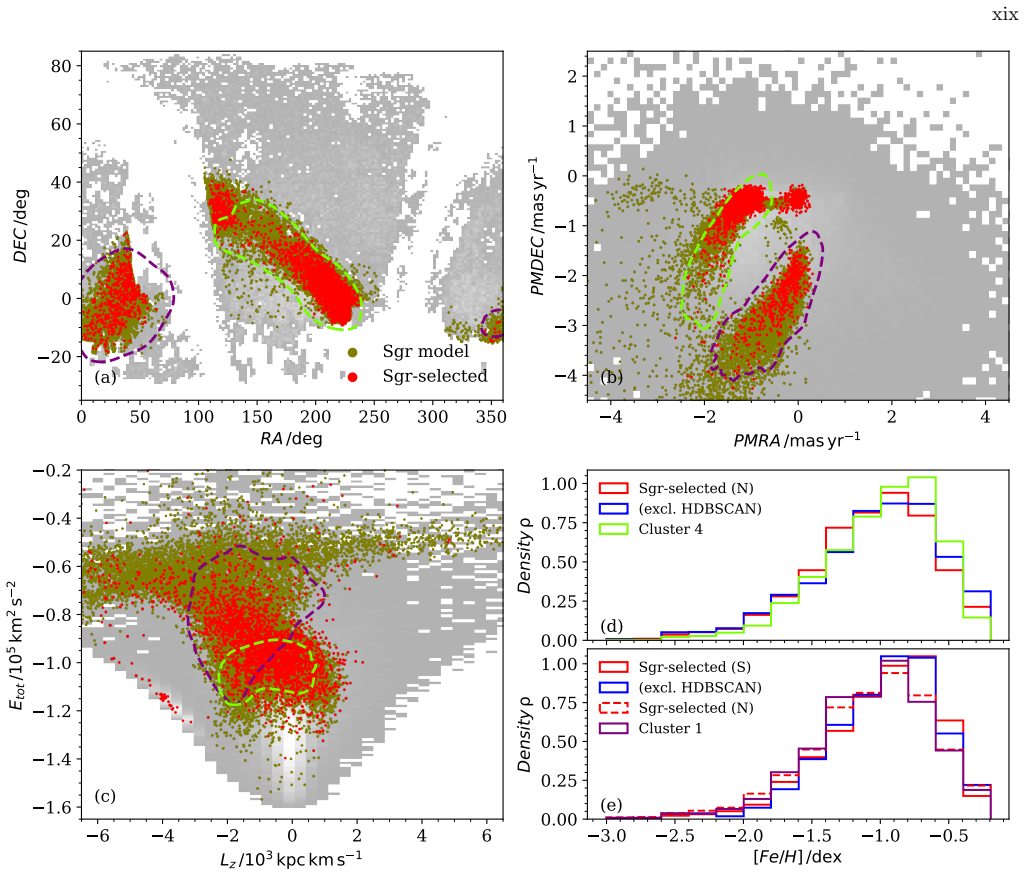
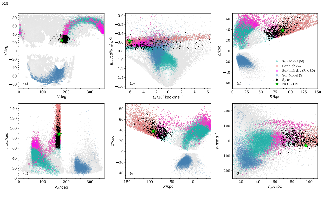
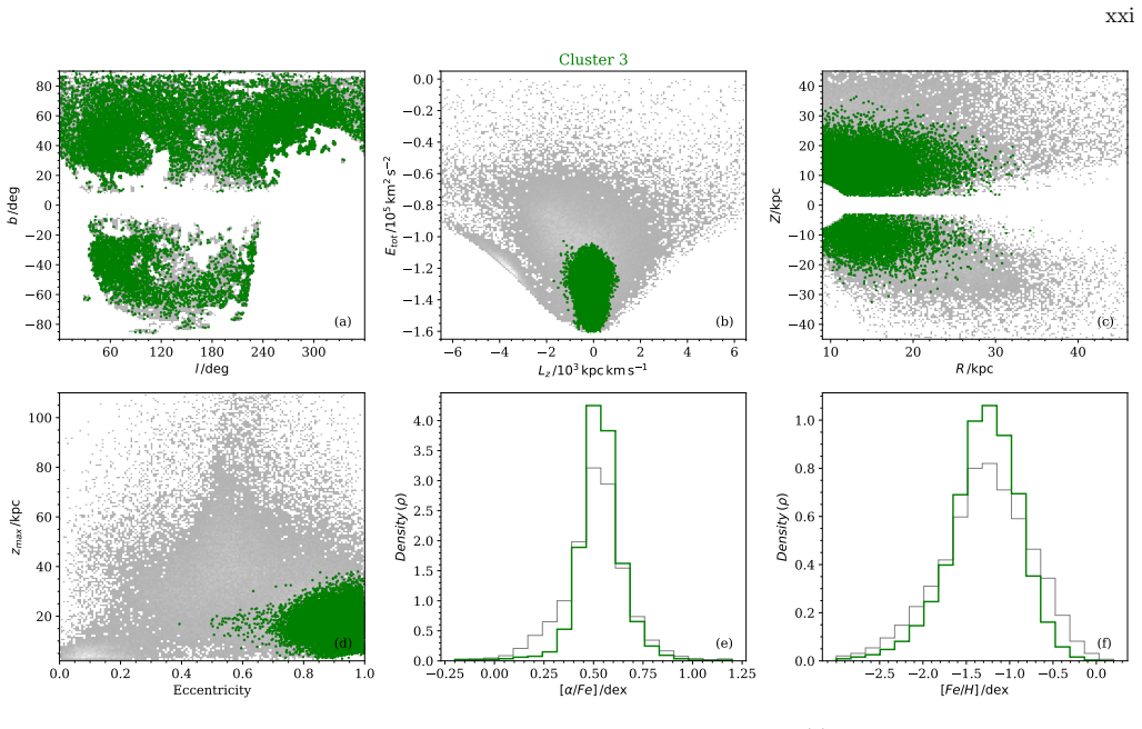
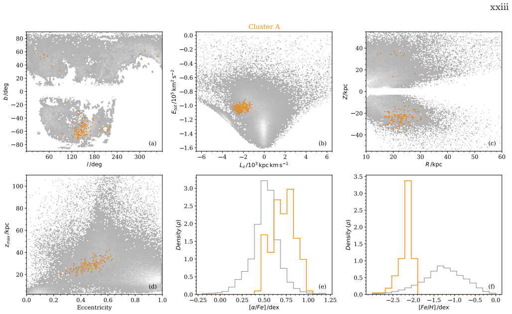
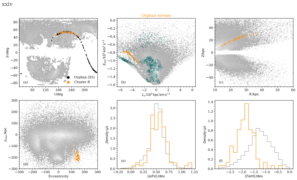
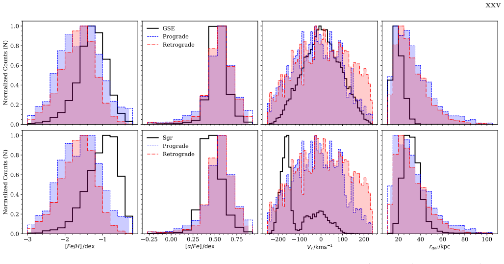
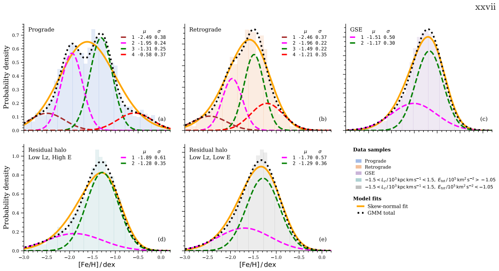
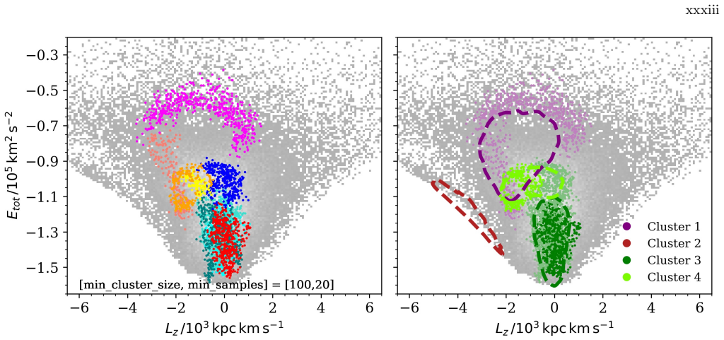
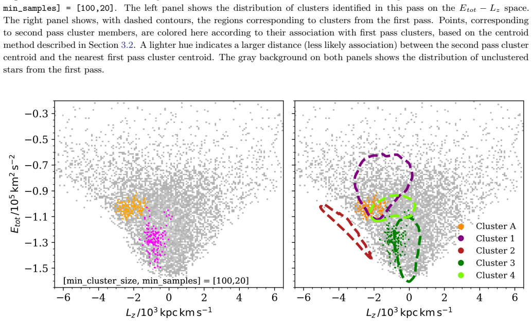
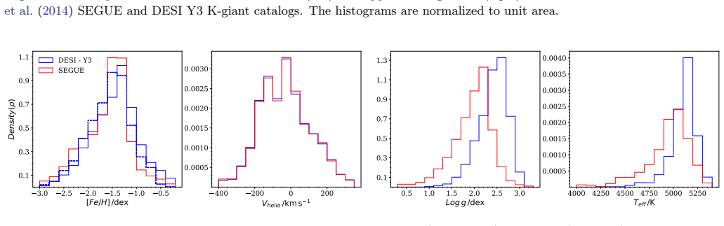
Using HDBSCAN on 6D phase-space and chemistry data from 88,959 K-giants, the authors identify substructures and isolate a residual halo. Samples of approximately 2000 outer halo stars with highly prograde and highly retrograde angular momenta exhibit similar metallicity distribution functions that are bimodal, with a metal-poor peak at [Fe/H] ~ -2 and a metal-rich peak at [Fe/H] ~ -1.3 for prograde or -1.5 for retrograde. These MDFs do not match those of GSE or Sagittarius. The lower angular momentum residual halo MDF resembles that of GSE even at lower binding energies.
What carries the argument
HDBSCAN clustering on 6D phase-space coordinates plus chemistry to separate known substructures from the residual stellar halo.
If this is right
- The residual halo MDFs are chemically distinct from both GSE and Sagittarius, implying contributions from additional accreted systems.
- Bimodality appears independently in both prograde and retrograde residual populations, indicating at least two chemically distinct components mixed across orbital directions.
- Lower-angular-momentum residual stars share an MDF shape with GSE at binding energies well below those of GSE itself.
- The outer halo is not dominated by a single massive merger at large radii.
Where Pith is reading between the lines
- The similarity of prograde and retrograde MDFs may indicate that the residual halo was assembled from several smaller satellites whose debris has phase-mixed in metallicity but not yet in orbit.
- Improved parallax or photometric distances from future surveys could test whether the reported bimodality survives when distance errors shrink.
- The GSE-like MDF at low angular momentum may trace either extended GSE debris or a separate but chemically similar progenitor.
- The residual halo MDF shape provides a new observable for testing whether the outer halo formed mainly through minor mergers after the GSE event.
Load-bearing premise
HDBSCAN clustering cleanly separates substructures from the residual halo without significant distance-induced contamination or parameter-dependent over- or under-clustering that would alter the reported MDF shapes.
What would settle it
Repeating the clustering and MDF measurement with tighter distance constraints or varied HDBSCAN parameters that removes the reported similarity or bimodality between the prograde and retrograde residual samples would falsify the central claim.
Figures
read the original abstract
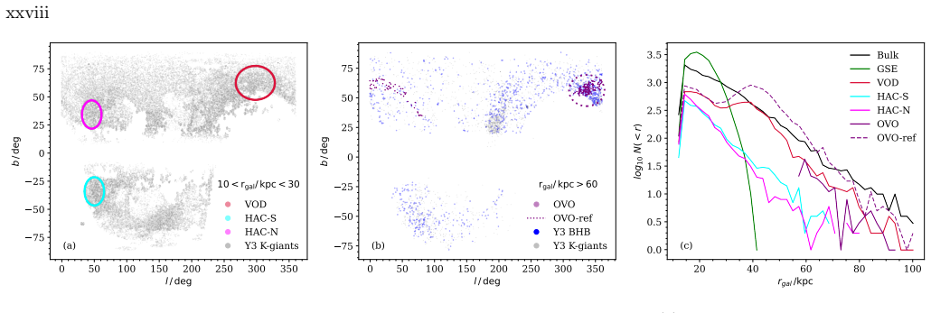
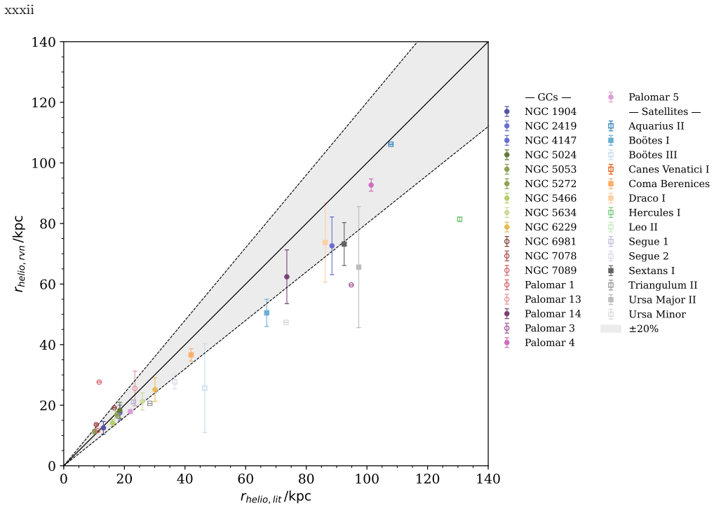
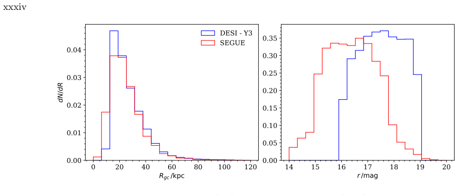
We present a sample of 88,959 K-giants from DESI Milky Way Survey Year 3 data, which we use to characterize the chemo-dynamical properties of the stellar halo at Galactocentric distances of 12 to ~100 kpc. Using HDBSCAN, we identify five prominent stellar halo substructures: Aleph, the Sagittarius stream, Gaia Sausage-Enceladus (GSE), Cetus-Palca and the Orphan-Chenab stream. We present the properties of each of these structures as they appear in our catalog, and examine how uncertainties on distance affect the characterization of substructure with this approach. We also examine regions associated with previously reported overdensities (such as the Virgo Overdensities and the Sagittarius spur) that we do not recover with HDBSCAN. The size and distance range of our catalog allows us to explore in detail the residual stellar halo, comprising stars that we do not associate with any substructure. We find that samples of ~2000 outer halo stars with both highly prograde and highly retrograde angular momenta have similar metallicity distribution functions (MDFs), which do not resemble the MDFs of either GSE or Sagittarius. Both the prograde and retrograde residual halo MDFs are bimodal, with a metal-poor peak at [Fe/H] ~ -2 and a metal-rich peak at [Fe/H] ~ -1.3 (prograde) or -1.5 (retrograde). The MDF for lower angular momentum residual halo K-giants does not show clear evidence for a metal-poor peak, and broadly resembles the MDF of GSE, even at much lower binding energies than GSE itself. We discuss possible interpretations of these findings for GSE accretion scenarios.
Editorial analysis
A structured set of objections, weighed in public.
Referee Report
Summary. The paper analyzes 88,959 K-giant stars from DESI Y3 data at 12-100 kpc, applies HDBSCAN to identify five substructures (Aleph, Sagittarius, GSE, Cetus-Palca, Orphan-Chenab), and characterizes the residual halo. It reports that ~2000 outer-halo stars with highly prograde and highly retrograde angular momenta exhibit similar bimodal MDFs (metal-poor peak at [Fe/H] ~ -2, metal-rich at -1.3/-1.5) that differ from GSE and Sgr, while lower-angular-momentum residual stars resemble GSE; implications for accretion scenarios are discussed.
Significance. If the residual-halo MDF bimodality and similarity hold after rigorous error propagation, the result constrains the Milky Way's accretion history by indicating that the distant residual halo contains distinct components beyond the dominant known mergers. The homogeneous, large-distance sample is a clear strength for halo studies.
major comments (3)
- [Abstract and residual-halo MDF section] The central claim that the prograde and retrograde residual-halo MDFs are bimodal and similar rests on clean HDBSCAN separation of the five substructures from the residual sample. Although the manuscript examines distance uncertainties for substructure characterization, it does not quantify how these uncertainties propagate into angular-momentum values, the 'highly prograde/retrograde' selection cuts, or the resulting MDF shapes for the ~2000-star samples (see abstract and the section on residual halo analysis).
- [Results section on substructure recovery] Post-hoc region definitions for previously reported overdensities (Virgo Overdensities, Sagittarius spur) that are not recovered by HDBSCAN are mentioned but their overlap with the residual halo and any effect on the reported bimodal MDFs remain unquantified.
- [Discussion section] The statement that the lower-angular-momentum residual-halo MDF resembles GSE 'even at much lower binding energies' requires explicit details on binding-energy calculation and a test of distance-error sensitivity, as this comparison underpins the discussion of GSE accretion scenarios.
minor comments (2)
- The exact numerical thresholds or cuts defining 'highly prograde' and 'highly retrograde' angular momenta should be stated explicitly (text or table) rather than left as qualitative descriptors.
- Figure captions for MDF panels should include the number of stars in each prograde/retrograde residual sample and the binning method used.
Simulated Author's Rebuttal
We thank the referee for their careful reading and constructive comments on our manuscript. We address each major comment below and will revise the paper accordingly to strengthen the analysis of uncertainties and provide additional details.
read point-by-point responses
-
Referee: [Abstract and residual-halo MDF section] The central claim that the prograde and retrograde residual-halo MDFs are bimodal and similar rests on clean HDBSCAN separation of the five substructures from the residual sample. Although the manuscript examines distance uncertainties for substructure characterization, it does not quantify how these uncertainties propagate into angular-momentum values, the 'highly prograde/retrograde' selection cuts, or the resulting MDF shapes for the ~2000-star samples (see abstract and the section on residual halo analysis).
Authors: We agree that propagation of distance uncertainties into the angular-momentum selection and MDFs of the residual halo samples was not quantified in detail, even though distance effects on substructure recovery were examined. We will add Monte Carlo realizations of distance errors to assess their impact on the Lz cuts and the resulting MDF shapes for the prograde and retrograde residual samples. revision: yes
-
Referee: [Results section on substructure recovery] Post-hoc region definitions for previously reported overdensities (Virgo Overdensities, Sagittarius spur) that are not recovered by HDBSCAN are mentioned but their overlap with the residual halo and any effect on the reported bimodal MDFs remain unquantified.
Authors: The post-hoc regions are noted for context, but we concur that their potential overlap with the residual halo and any contribution to the bimodal MDFs should be quantified. We will add an assessment of the stellar fractions in these regions that enter the residual sample and evaluate their effect on the reported MDFs. revision: yes
-
Referee: [Discussion section] The statement that the lower-angular-momentum residual-halo MDF resembles GSE 'even at much lower binding energies' requires explicit details on binding-energy calculation and a test of distance-error sensitivity, as this comparison underpins the discussion of GSE accretion scenarios.
Authors: We will include the explicit binding-energy formula and computation method in the revised text. We will also add a distance-error sensitivity test for the lower-angular-momentum residual sample to confirm the robustness of the MDF resemblance to GSE. revision: yes
Circularity Check
No significant circularity; purely observational measurements
full rationale
The paper reports direct empirical measurements of MDFs from DESI K-giant catalog data after applying HDBSCAN clustering to identify and remove substructures. No derivations, fitted parameters renamed as predictions, self-citation chains, or ansatzes are present in the load-bearing steps. The central claims about bimodal MDF shapes in prograde/retrograde residual halo samples are computed directly from the selected stars without reduction to inputs by construction. This is self-contained observational analysis.
Axiom & Free-Parameter Ledger
Reference graph
Works this paper leans on
-
[1]
Abadi, M. G., Navarro, J. F., & Steinmetz, M. 2006, MNRAS, 365, 747 Abdul Karim, M., Aguilar, J., Ahlen, S., et al. 2025, PhRvD, 112, 083515, doi: 10.1103/tr6y-kpc6
-
[2]
Aganze, C., Chandra, V., Wechsler, R. H., et al. 2025, arXiv e-prints, arXiv:2504.11687, doi: 10.48550/arXiv.2504.11687 Allende Prieto, C., Beers, T. C., Wilhelm, R., et al. 2006, ApJ, 636, 804, doi: 10.1086/498131 Allende Prieto, C., Cooper, A. P., Dey, A., et al. 2020, Research Notes of the American Astronomical Society, 4, 188, doi: 10.3847/2515-5172/abc1dc
-
[3]
Laporte, C. F. P., & Deg, N. 2022, ApJ, 937, 12, doi: 10.3847/1538-4357/ac8b0d
-
[4]
Amarante, J. A. S., Koposov, S. E., & Laporte, C. F. P. 2024, A&A, 690, A166
2024
-
[5]
Amorisco, N. C. 2017, MNRAS, 464, 2882 Astropy Collaboration, Robitaille, T. P., Tollerud, E. J., et al. 2013, A&A, 558, A33, doi: 10.1051/0004-6361/201322068 Astropy Collaboration, Price-Whelan, A. M., Sipőcz, B. M., et al. 2018, AJ, 156, 123, doi: 10.3847/1538-3881/aabc4f Astropy Collaboration, Price-Whelan, A. M., Lim, P. L., et al. 2022, ApJ, 935, 167...
-
[6]
2021, MNRAS, 505, 5957, doi: 10.1093/mnras/stab1474
Baumgardt, H., & Vasiliev, E. 2021, MNRAS, 505, 5957, doi: 10.1093/mnras/stab1474
-
[7]
Bayer, M., Starkenburg, E., Thomas, G. F., et al. 2025, A&A, 701, A117, doi: 10.1051/0004-6361/202554131
-
[8]
F., Zucker, D
Bell, E. F., Zucker, D. B., Belokurov, V., et al. 2008, ApJ, 680, 295
2008
-
[9]
Deason, A. J. 2018, MNRAS, 478, 611, doi: 10.1093/mnras/sty982
-
[10]
2023, MNRAS, 525, 4456
Belokurov, V., & Kravtsov, A. 2023, MNRAS, 525, 4456
2023
-
[11]
W., Bell, E
Belokurov, V., Evans, N. W., Bell, E. F., et al. 2007, ApJL, 657, L89
2007
-
[12]
Belokurov, V., Koposov, S. E., Evans, N. W., et al. 2014, MNRAS, 437, 116, doi: 10.1093/mnras/stt1862
-
[13]
2019, MNRAS, 482, 1417, doi: 10.1093/mnras/sty2813
Bennett, M., & Bovy, J. 2019, MNRAS, 482, 1417, doi: 10.1093/mnras/sty2813
work page internal anchor Pith review doi:10.1093/mnras/sty2813 2019
-
[14]
2025, A&A, 700, A160, doi: 10.1051/0004-6361/202555272
Berni, L., Spina, L., Magrini, L., et al. 2025, A&A, 700, A160, doi: 10.1051/0004-6361/202555272
-
[15]
A., Xue, X.-X., Liu, C., et al
Bird, S. A., Xue, X.-X., Liu, C., et al. 2019, AJ, 157, 104, doi: 10.3847/1538-3881/aafd2e —. 2022, MNRAS, 516, 731, doi: 10.1093/mnras/stac2036
-
[16]
Blanton, M. R., Bershady, M. A., Abolfathi, B., et al. 2017, AJ, 154, 28, doi: 10.3847/1538-3881/aa7567
-
[17]
Borbolato, L., Perottoni, H. D., Rossi, S., et al. 2024, ApJ, 960, 52, doi: 10.3847/1538-4357/ad02fb
-
[18]
Brauer, K., Andales, H. D., Ji, A. P., et al. 2022, ApJ, 937, 14, doi: 10.3847/1538-4357/ac85b9
-
[19]
2021, MNRAS, 506, 150, doi: 10.1093/mnras/stab1242
Buder, S., Sharma, S., Kos, J., et al. 2021, MNRAS, 506, 150, doi: 10.1093/mnras/stab1242
-
[20]
S., & Johnston, K
Bullock, J. S., & Johnston, K. V. 2005, ApJ, 635, 931
2005
-
[21]
S., Kravtsov, A
Bullock, J. S., Kravtsov, A. V., & Weinberg, D. H. 2001, ApJ, 548, 33 Byström, A., Koposov, S. E., Lilleengen, S., et al. 2025, MNRAS, 542, 560
2001
-
[22]
Campello, R. J. G. B., Moulavi, D., & Sander, J. 2013, in Advances in Knowledge Discovery and Data Mining, ed. J. Pei, V. S. Tseng, L. Cao, H. Motoda, & G. Xu (Berlin, Heidelberg: Springer Berlin Heidelberg), 160–172
2013
-
[23]
L., Liu, C., Newberg, H
Carlin, J. L., Liu, C., Newberg, H. J., et al. 2016, ApJ, 822, 16
2016
-
[24]
Carollo, D., Beers, T. C., Chiba, M., et al. 2010, ApJ, 712, 692, doi: 10.1088/0004-637X/712/1/692
-
[25]
2019, ApJ, 887, 22, doi: 10.3847/1538-4357/ab517c
Carollo, D., Chiba, M., Ishigaki, M., et al. 2019, ApJ, 887, 22, doi: 10.3847/1538-4357/ab517c
-
[26]
J., Fattahi, A., Callingham, T
Carrillo, A., Deason, A. J., Fattahi, A., Callingham, T. M., & Grand, R. J. J. 2024, MNRAS, 527, 2165, doi: 10.1093/mnras/stad3274
-
[27]
P., Conroy, C., et al
Chandra, V., Naidu, R. P., Conroy, C., et al. 2023, ApJ, 951, 26 xxxvi
2023
-
[28]
Chandra, V., Cargile, P. A., Ji, A. P., et al. 2026, ApJ, 1000, 283, doi: 10.3847/1538-4357/ae448a
-
[29]
2020, ApJ, 905, 100, doi: 10.3847/1538-4357/abc338
Chang, J., Yuan, Z., Xue, X.-X., et al. 2020, ApJ, 905, 100, doi: 10.3847/1538-4357/abc338
-
[30]
Chiba, M., & Beers, T. C. 2000, AJ, 119, 2843, doi: 10.1086/301409
-
[31]
1998, AJ, 115, 168, doi: 10.1086/300177
Chiba, M., & Yoshii, Y. 1998, AJ, 115, 168, doi: 10.1086/300177
-
[32]
2019, ApJ, 883, 107, doi: 10.3847/1538-4357/ab38b8
Conroy, C., Bonaca, A., Cargile, P., et al. 2019, ApJ, 883, 107, doi: 10.3847/1538-4357/ab38b8
-
[33]
P., Parry, O
Cooper, A. P., Parry, O. H., Lowing, B., Cole, S., & Frenk, C. 2015, MNRAS, 454, 3185
2015
-
[34]
Cooper, A. P., Cole, S., Frenk, C. S., et al. 2010, MNRAS, 406, 744, doi: 10.1111/j.1365-2966.2010.16740.x
-
[35]
Cooper, A. P., Koposov, S. E., Allende Prieto, C., et al. 2023, ApJ, 947, 37, doi: 10.3847/1538-4357/acb3c0
-
[36]
Cui, X.-Q., Zhao, Y.-H., Chu, Y.-Q., et al. 2012, Research in Astronomy and Astrophysics, 12, 1197, doi: 10.1088/1674-4527/12/9/003
-
[37]
Cunningham, E. C., Hunt, J. A. S., Price-Whelan, A. M., et al. 2024, ApJ, 963, 95, doi: 10.3847/1538-4357/ad187b
-
[38]
and Belokurov, Vasily and Monty, Stephanie and Evans, N
Davies, E. Y., Belokurov, V., Monty, S., & Evans, N. W. 2024, MNRAS, 529, L73, doi: 10.1093/mnrasl/slae001 De Silva, G. M., Freeman, K. C., Bland-Hawthorn, J., et al. 2015, MNRAS, 449, 2604, doi: 10.1093/mnras/stv327
-
[39]
Deason, A. J., & Belokurov, V. 2024, NewAR, 99, 101706, doi: 10.1016/j.newar.2024.101706
-
[40]
J., Belokurov, V., Koposov, S
Deason, A. J., Belokurov, V., Koposov, S. E., et al. 2017, ArXiv e-prints
2017
-
[41]
J., Belokurov, V., Koposov, S
Deason, A. J., Belokurov, V., Koposov, S. E., & Lancaster, L. 2018, ArXiv e-prints
2018
-
[42]
The DESI Experiment Part I: Science,Targeting, and Survey Design
Deason, A. J., Belokurov, V., & Sanders, J. L. 2019, MNRAS, 490, 3426 DESI Collaboration, Aghamousa, A., Aguilar, J., et al. 2016a, arXiv e-prints, arXiv:1611.00036, doi: 10.48550/arXiv.1611.00036 —. 2016b, arXiv e-prints, arXiv:1611.00037, doi: 10.48550/arXiv.1611.00037 DESI Collaboration, Abareshi, B., Aguilar, J., et al. 2022, AJ, 164, 207, doi: 10.384...
work page internal anchor Pith review Pith/arXiv arXiv doi:10.48550/arxiv.1611.00036 2019
-
[43]
Dey, A., Schlegel, D. J., Lang, D., et al. 2019, AJ, 157, 168, doi: 10.3847/1538-3881/ab089d
-
[44]
Dey, A., Koposov, S. E., Najita, J. R., et al. 2025, arXiv e-prints, arXiv:2505.17230. https://arxiv.org/abs/2505.17230
arXiv 2025
-
[45]
M., Belokurov, V., Font, A
Dillamore, A. M., Belokurov, V., Font, A. S., & McCarthy, I. G. 2022, MNRAS, 513, 1867
2022
-
[46]
Dillamore, A. M., & Sanders, J. L. 2025, MNRAS, 542, 1331, doi: 10.1093/mnras/staf1264
-
[47]
2025, Research in Astronomy and Astrophysics, 25, 095015, doi: 10.1088/1674-4527/ade522
Ding, L., Li, J., Xue, X.-X., et al. 2025, Research in Astronomy and Astrophysics, 25, 095015, doi: 10.1088/1674-4527/ade522
-
[48]
M., Helmi, A., et al
Dodd, E., Callingham, T. M., Helmi, A., et al. 2023, A&A, 670, L2
2023
-
[49]
C., Helmi, A., Morrison, H., et al
Dohm-Palmer, R. C., Helmi, A., Morrison, H., et al. 2001, ApJL, 555, L37, doi: 10.1086/321734
-
[50]
Donlon, T., Newberg, H. J., Sanderson, R., et al. 2024, MNRAS, 531, 1422, doi: 10.1093/mnras/stae1264
-
[51]
Donlon, II, T., Newberg, H. J., Kim, B., & Lépine, S. 2022, ApJL, 932, L16, doi: 10.3847/2041-8213/ac7531
-
[52]
J., Sanderson, R., & Widrow, L
Donlon, II, T., Newberg, H. J., Sanderson, R., & Widrow, L. M. 2020, ApJ, 902, 119, doi: 10.3847/1538-4357/abb5f6
-
[53]
J., Catelan, M., Djorgovski, S
Drake, A. J., Catelan, M., Djorgovski, S. G., et al. 2013, ApJ, 765, 154
2013
-
[54]
2018, Research Notes of the American Astronomical Society, 2, 210, doi: 10.3847/2515-5172/aaef8b
Drimmel, R., & Poggio, E. 2018, Research Notes of the American Astronomical Society, 2, 210, doi: 10.3847/2515-5172/aaef8b
-
[55]
Eisenstein, D. J., Weinberg, D. H., Agol, E., et al. 2011, AJ, 142, 72, doi: 10.1088/0004-6256/142/3/72
-
[56]
Evans, N. W. 2020, in IAU Symposium, Vol. 353, Galactic Dynamics in the Era of Large Surveys, ed. M. Valluri & J. A. Sellwood, 113–120
2020
-
[57]
Fattahi, A., Belokurov, V., Deason, A. J., et al. 2019, MNRAS, 484, 4471, doi: 10.1093/mnras/stz159
-
[58]
2025, ApJ, 983, 119, doi: 10.3847/1538-4357/adbe31 Gaia Collaboration, Prusti, T., de Bruijne, J
Folsom, D., Lisanti, M., Necib, L., et al. 2025, ApJ, 983, 119, doi: 10.3847/1538-4357/adbe31 Gaia Collaboration, Prusti, T., de Bruijne, J. H. J., et al. 2016, A&A, 595, A1, doi: 10.1051/0004-6361/201629272 Gaia Collaboration, Brown, A. G. A., Vallenari, A., et al. 2018, A&A, 616, A1, doi: 10.1051/0004-6361/201833051 —. 2021, A&A, 649, A1, doi: 10.1051/0...
-
[59]
Gunn, J. E., Siegmund, W. A., Mannery, E. J., et al. 2006, AJ, 131, 2332, doi: 10.1086/500975
-
[60]
D., Preibisch, T., & Minniti, D
Gupta, A., Ivanov, V. D., Preibisch, T., & Minniti, D. 2024, A&A, 692, A194, doi: 10.1051/0004-6361/202451078
-
[61]
Guy, J., Bailey, S., Kremin, A., et al. 2023, AJ, 165, 144, doi: 10.3847/1538-3881/acb212 xxxvii
-
[62]
Hahn, C., Wilson, M. J., Ruiz-Macias, O., et al. 2023, AJ, 165, 253, doi: 10.3847/1538-3881/accff8
-
[63]
Han, J. J., Conroy, C., Johnson, B. D., et al. 2022, AJ, 164, 249, doi: 10.3847/1538-3881/ac97e9
-
[64]
Harris, C. R., Millman, K. J., van der Walt, S. J., et al. 2020, Nature, 585, 357, doi: 10.1038/s41586-020-2649-2
-
[65]
2020, ARA&A, 58, 205, doi: 10.1146/annurev-astro-032620-021917
Helmi, A. 2020, ARA&A, 58, 205, doi: 10.1146/annurev-astro-032620-021917
-
[66]
Helmi, A., Babusiaux, C., Koppelman, H. H., et al. 2018, Nature, 563, 85, doi: 10.1038/s41586-018-0625-x
-
[67]
Helmi, A., & de Zeeuw, P. T. 2000, MNRAS, 319, 657, doi: 10.1046/j.1365-8711.2000.03895.x
-
[68]
Helmi, A., & White, S. D. M. 1999, MNRAS, 307, 495
1999
-
[69]
Helmi, A., White, S. D. M., de Zeeuw, P. T., & Zhao, H. 1999, Nature, 402, 53, doi: 10.1038/46980
-
[70]
Holtzman, J. A., Shetrone, M., Johnson, J. A., et al. 2015, AJ, 150, 148, doi: 10.1088/0004-6256/150/5/148
-
[71]
Hong, J., Beers, T. C., Lee, Y. S., et al. 2024, ApJS, 273, 12, doi: 10.3847/1538-4365/ad4a6f
-
[72]
Horta, D., & Schiavon, R. P. 2024, Ap&SS, 369, 107, doi: 10.1007/s10509-024-04370-y
-
[73]
Horta, D., Schiavon, R. P., Mackereth, J. T., et al. 2023, MNRAS, 520, 5671, doi: 10.1093/mnras/stac3179
-
[74]
Huang, Y., Liu, X. W., Yuan, H. B., et al. 2016, MNRAS, 463, 2623, doi: 10.1093/mnras/stw2096
-
[75]
Hunt, E. L., & Reffert, S. 2021, A&A, 646, A104, doi: 10.1051/0004-6361/202039341
-
[76]
Hunter, J. D. 2007, Computing in Science & Engineering, 9, 90, doi: 10.1109/MCSE.2007.55
-
[77]
Ibata, R. A., Gilmore, G., & Irwin, M. J. 1994, Nature, 370, 194, doi: 10.1038/370194a0
-
[78]
2019, MNRAS, 482, 3868 Ivezić, Ž., Sesar, B., Jurić, M., et al
Iorio, G., & Belokurov, V. 2019, MNRAS, 482, 3868 Ivezić, Ž., Sesar, B., Jurić, M., et al. 2008, ApJ, 684, 287
2019
-
[79]
Janesh, W., Morrison, H. L., Ma, Z., et al. 2016, ApJ, 816, 80, doi: 10.3847/0004-637X/816/2/80
-
[80]
2017, A&A, 604, A106, doi: 10.1051/0004-6361/201629691
Jean-Baptiste, I., Di Matteo, P., Haywood, M., et al. 2017, A&A, 604, A106, doi: 10.1051/0004-6361/201629691
discussion (0)
Sign in with ORCID, Apple, or X to comment. Anyone can read and Pith papers without signing in.