Characterization of Numerical Dissipation in Simulations of Magnetohydrodynamic Turbulence
Pith reviewed 2026-06-26 09:45 UTC · model grok-4.3
The pith
A framework estimates numerical dissipation in MHD turbulence simulations directly from data without prior assumptions on its form.
A machine-rendered reading of the paper's core claim, the machinery that carries it, and where it could break.
Core claim
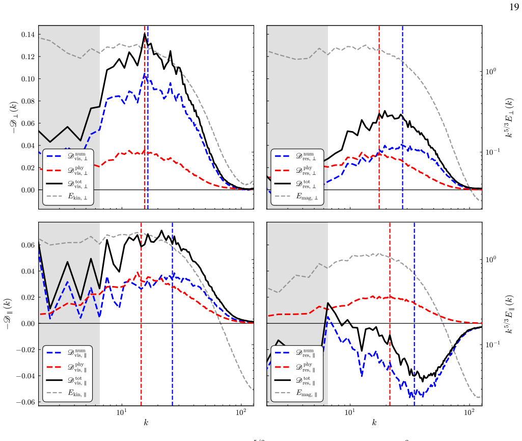
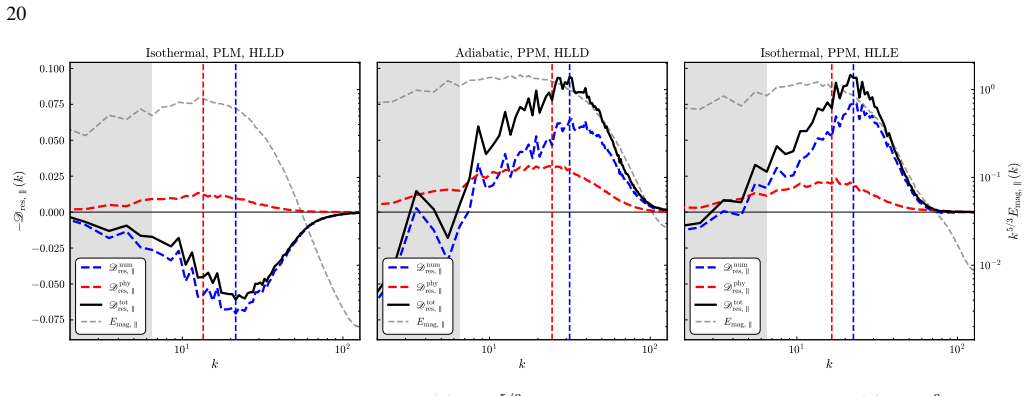
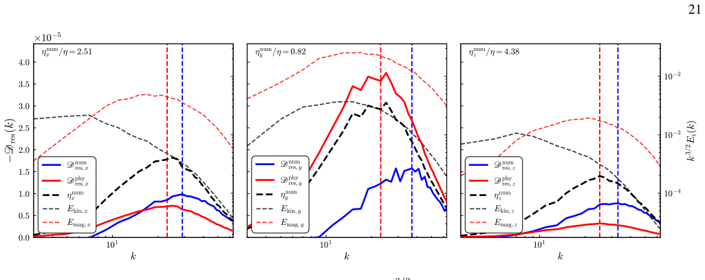
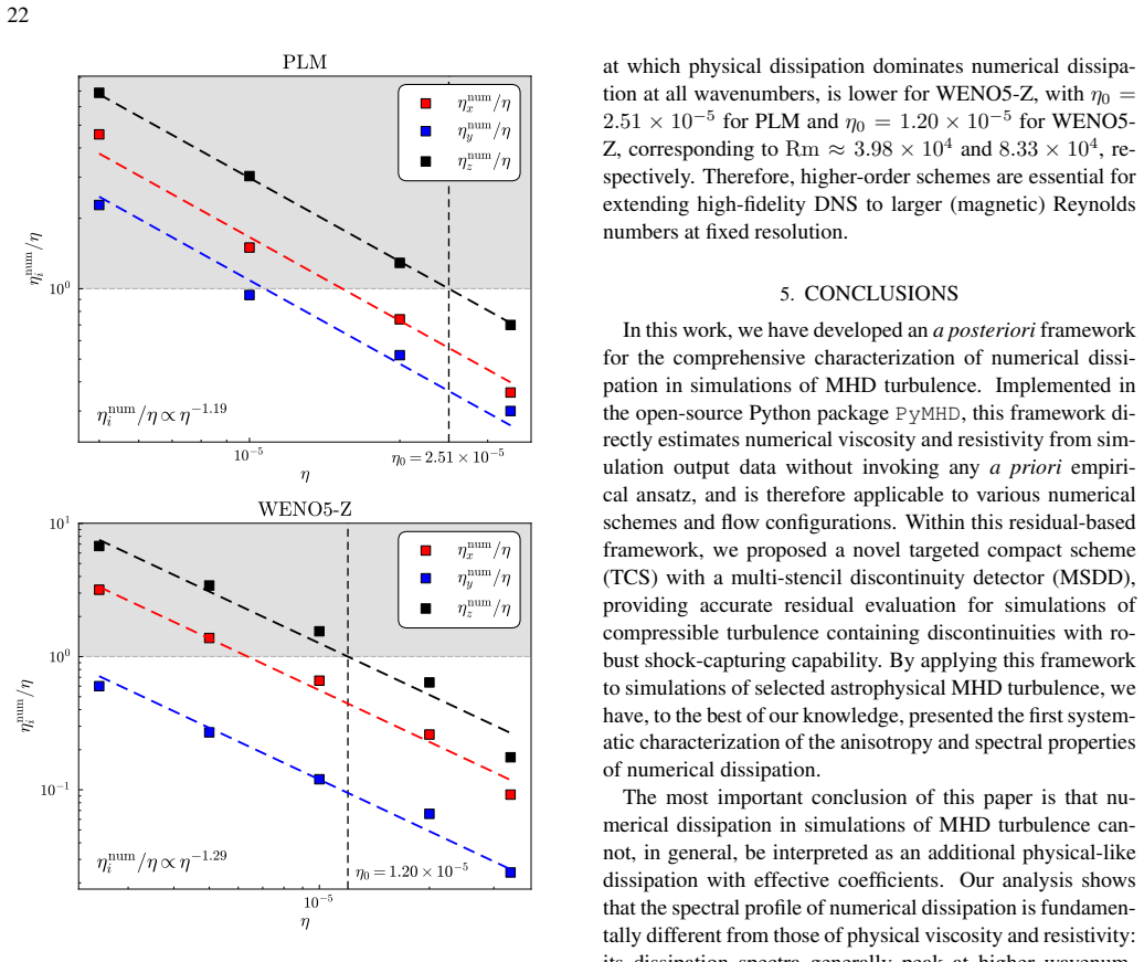
We present an a posteriori framework for directly estimating numerical dissipation in MHD turbulence from simulation data without invoking a priori assumptions. Implemented in the open-source Python package PyMHD, the framework is applied to simulations of Alfvénic turbulence, turbulent small-scale dynamos, and MRI-driven turbulence, yielding a systematic characterization of the anisotropy and spectral properties of numerical dissipation across these regimes. The results indicate that numerical dissipation primarily dissipates energy transferred by the turbulent cascade at small scales, consistent with the conventional interpretation. However, its spectral properties are distinct from those
What carries the argument
an a posteriori framework for directly estimating numerical dissipation from simulation data
If this is right
- Numerical dissipation primarily dissipates energy transferred by the turbulent cascade at small scales.
- Its spectral properties are distinct from physical viscosity and resistivity so it cannot be represented by effective dissipation coefficients.
- Numerical dissipation inherits the anisotropy of the underlying turbulence.
- Numerical dissipation can exhibit anomalous anti-dissipative behavior under certain circumstances.
- The framework identifies conditions under which physical dissipation dominates numerical dissipation across all scales.
Where Pith is reading between the lines
- The same data-driven separation approach could be tested on non-MHD fluid turbulence simulations to check generality.
- If the framework succeeds, it supplies a practical test for whether a given grid resolution makes physical dissipation dominant in a target astrophysical regime.
- Regime-specific anisotropy in numerical dissipation may require different resolution strategies depending on the type of MHD turbulence being modeled.
Load-bearing premise
That the post-simulation data alone contains sufficient information to separate numerical dissipation from physical effects and from the turbulent cascade without any modeling assumptions about the form of dissipation.
What would settle it
A calculation showing that the framework's estimated numerical dissipation rate does not match the observed total energy loss rate in a high-resolution simulation where physical dissipation is set to zero would falsify the separation claim.
Figures
read the original abstract
Comprehensive characterization of numerical dissipation is essential for high-fidelity simulations of magnetohydrodynamic (MHD) turbulence. In this work, we present an a posteriori framework for directly estimating numerical dissipation in MHD turbulence from simulation data without invoking a priori assumptions. Implemented in the open-source Python package PyMHD, the framework is applied to simulations of Alfv\'enic turbulence, turbulent small-scale dynamos, and MRI-driven turbulence, yielding a systematic characterization of the anisotropy and spectral properties of numerical dissipation across these regimes. The results indicate that numerical dissipation primarily dissipates energy transferred by the turbulent cascade at small scales, consistent with the conventional interpretation. However, its spectral properties are distinct from those of physical viscosity and resistivity, such that it cannot simply be represented by effective dissipation coefficients. In addition, numerical dissipation inherits the anisotropy of the underlying turbulence, and can even exhibit anomalous anti-dissipative behavior under certain circumstances. Moreover, this framework enables identification of the conditions under which physical dissipation dominates numerical dissipation across all scales, thereby providing practical guidance for achieving high-fidelity simulations of astrophysical MHD turbulence.
Editorial analysis
A structured set of objections, weighed in public.
Referee Report
Summary. The manuscript presents an a posteriori framework, implemented in the open-source PyMHD package, for directly estimating numerical dissipation in MHD turbulence simulations from post-simulation data without a priori assumptions. The framework is applied to Alfvénic turbulence, turbulent small-scale dynamos, and MRI-driven turbulence to characterize the anisotropy and spectral properties of numerical dissipation, with findings that it primarily acts on energy transferred by the turbulent cascade at small scales, exhibits distinct spectral properties from physical viscosity/resistivity, inherits turbulence anisotropy, and can display anomalous anti-dissipative behavior; it also identifies regimes where physical dissipation dominates.
Significance. If the framework reliably isolates numerical dissipation without implicit modeling assumptions, the work would be significant for guiding high-fidelity astrophysical MHD simulations by clarifying when numerical effects can be neglected versus when they contaminate results. The open-source implementation and systematic application across three distinct regimes are positive features that could aid reproducibility and practical use.
major comments (3)
- [Abstract and framework description (likely §2–3)] Abstract and framework description (likely §2–3): the load-bearing claim that the estimator operates 'without invoking a priori assumptions' and separates numerical dissipation from the turbulent cascade and physical dissipation is not secured by the presented evidence. Any concrete implementation via filtered energy budgets or scale-local balances requires operational choices (filtering scale, stationarity criteria, or expected cascade shape) that encode modeling assumptions; the reported anomalous anti-dissipative behavior indicates the estimator can produce results outside conventional models, yet no explicit validation is described that varies physical viscosity/resistivity independently while holding the numerical scheme fixed to demonstrate unbiased recovery of numerical dissipation.
- [Results sections on spectral properties (likely §4–5)] Results sections on spectral properties (likely §4–5): the claim that numerical dissipation 'cannot simply be represented by effective dissipation coefficients' because its spectral properties are distinct rests on the estimator definition, but without quantitative comparison to controlled cases (e.g., varying grid resolution or explicit physical coefficients) or derivation showing the estimator remains unbiased, it is unclear whether the distinction arises from true numerical behavior or from the method's construction. An equation-level derivation of the estimator (e.g., the precise form of the numerical dissipation term extracted from the energy budget) is needed to assess this.
- [Application to MRI-driven turbulence and anti-dissipative regimes (likely §5.3)] Application to MRI-driven turbulence and anti-dissipative regimes (likely §5.3): the observation of anomalous anti-dissipative behavior is a striking result that challenges conventional expectations, but it is load-bearing for the framework's reliability; without additional tests (e.g., convergence with resolution or cross-check against known analytic limits), this risks indicating an artifact of the separation procedure rather than a physical/numerical feature.
minor comments (2)
- [Abstract] The abstract would benefit from a one-sentence summary of the precise operational definition used for the numerical dissipation estimator to allow readers to assess the 'no a priori assumptions' claim immediately.
- [Figures (throughout results)] Figure captions and axis labels in the spectral and anisotropy plots should explicitly state the normalization and any filtering parameters employed, to improve clarity for readers reproducing the results.
Simulated Author's Rebuttal
We thank the referee for their constructive comments on our manuscript. We address each of the major comments below, providing clarifications and indicating where revisions will be made to improve the presentation and rigor of the work.
read point-by-point responses
-
Referee: Abstract and framework description (likely §2–3): the load-bearing claim that the estimator operates 'without invoking a priori assumptions' and separates numerical dissipation from the turbulent cascade and physical dissipation is not secured by the presented evidence. Any concrete implementation via filtered energy budgets or scale-local balances requires operational choices (filtering scale, stationarity criteria, or expected cascade shape) that encode modeling assumptions; the reported anomalous anti-dissipative behavior indicates the estimator can produce results outside conventional models, yet no explicit validation is described that varies physical viscosity/resistivity independently while holding the numerical scheme fixed to demonstrate unbiased recovery of numerical dissipation.
Authors: We agree that operational choices such as the filtering scale are necessary in any practical implementation. However, the core of the framework is to compute the numerical dissipation as the residual in the energy budget after subtracting all explicitly resolved terms (including physical dissipation where present), without assuming a functional form for the numerical term itself. This is distinct from a priori modeling. We did not perform the suggested validation test of varying physical coefficients while fixing the numerical scheme, as our focus was on characterizing numerical effects in typical simulation setups. We will revise the manuscript to explicitly discuss these operational choices and their potential impact, and add a derivation of the estimator from the filtered MHD equations. revision: partial
-
Referee: Results sections on spectral properties (likely §4–5): the claim that numerical dissipation 'cannot simply be represented by effective dissipation coefficients' because its spectral properties are distinct rests on the estimator definition, but without quantitative comparison to controlled cases (e.g., varying grid resolution or explicit physical coefficients) or derivation showing the estimator remains unbiased, it is unclear whether the distinction arises from true numerical behavior or from the method's construction. An equation-level derivation of the estimator (e.g., the precise form of the numerical dissipation term extracted from the energy budget) is needed to assess this.
Authors: We acknowledge the need for an equation-level derivation to make the estimator transparent. The numerical dissipation term is obtained by rearranging the filtered energy equation: the time derivative and advection terms are computed from the data, physical dissipation is subtracted if known, and the residual is attributed to numerical effects. This will be added to §2 or §3. Regarding quantitative comparisons, our applications across different resolutions in the Alfvénic and dynamo cases show consistent spectral shapes distinct from physical dissipation. We will include additional discussion comparing to cases with explicit dissipation to support the claim. revision: yes
-
Referee: Application to MRI-driven turbulence and anti-dissipative regimes (likely §5.3): the observation of anomalous anti-dissipative behavior is a striking result that challenges conventional expectations, but it is load-bearing for the framework's reliability; without additional tests (e.g., convergence with resolution or cross-check against known analytic limits), this risks indicating an artifact of the separation procedure rather than a physical/numerical feature.
Authors: This is an important point. The anti-dissipative behavior appears in specific parameter regimes of the MRI simulations where the turbulent cascade is strong. We have checked that it persists across the available resolutions, but agree that more explicit convergence tests would be beneficial. We will add a subsection discussing the resolution dependence for the MRI cases and note that this behavior may indicate backscatter or inverse cascade effects captured by the estimator. If this is an artifact, it would be valuable to identify, but our current data supports it as a feature in those regimes. revision: partial
Circularity Check
No significant circularity; framework presented as data-driven without shown self-referential reductions
full rationale
The provided abstract and context describe an a posteriori framework that estimates numerical dissipation directly from simulation data without a priori assumptions. No equations, fitted parameters renamed as predictions, or self-citation chains are quoted that would reduce the central claim to its inputs by construction. The derivation is presented as self-contained, relying on post-simulation fields to characterize dissipation properties across regimes. This matches the default expectation of no circularity when no explicit reduction is exhibited.
Axiom & Free-Parameter Ledger
Reference graph
Works this paper leans on
-
[1]
2021, Physical Review Letters, 126, doi: 10.1103/physrevlett.126.091103 Anthropic
Achikanath Chirakkara, R., Federrath, C., Trivedi, P., & Banerjee, R. 2021, Physical Review Letters, 126, doi: 10.1103/physrevlett.126.091103 Anthropic. 2026, Claude Opus 4.8 System Card, Tech. rep., Anthropic. https://www.anthropic.com/claude-opus-4-8-system-card
-
[2]
Balbus, S. A., & Hawley, J. F. 1991, The Astrophysical Journal, 376, 214, doi: 10.1086/170270
-
[3]
title Instability, turbulence, and enhanced transport in accretion disks
Balbus, S. A., & Hawley, J. F. 1998, Reviews of Modern Physics, 70, 1, doi: 10.1103/revmodphys.70.1
-
[4]
Balsara, D. S., & Shu, C.-W. 2000, Journal of Computational Physics, 160, 405, doi: 10.1006/jcph.2000.6443
-
[5]
2025, Nature Astronomy, 9, 1195, doi: 10.1038/s41550-025-02551-5
Bhattacharjee, A. 2025, Nature Astronomy, 9, 1195, doi: 10.1038/s41550-025-02551-5
-
[6]
2012, Physical Review Letters, 108, doi: 10.1103/physrevlett.108.035002
Beresnyak, A. 2012, Physical Review Letters, 108, doi: 10.1103/physrevlett.108.035002
-
[7]
2003, Magnetohydrodynamic Turbulence (Cambridge University Press), doi: 10.1017/cbo9780511535222
Biskamp, D. 2003, Magnetohydrodynamic Turbulence (Cambridge University Press), doi: 10.1017/cbo9780511535222
-
[8]
Borges, R., Carmona, M., Costa, B., & Don, W. S. 2008, Journal of Computational Physics, 227, 3191, doi: 10.1016/j.jcp.2007.11.038
-
[9]
Boris, J. P., Grinstein, F. F., Oran, E. S., & Kolbe, R. L. 1992, Fluid Dynamics Research, 10, 199, doi: 10.1016/0169-5983(92)90023-p
-
[10]
Bott, A. F. A., Chen, L., Boutoux, G., et al. 2021, Physical Review Letters, 127, doi: 10.1103/physrevlett.127.175002
-
[11]
Bott, A. F. A., Chen, L., Tzeferacos, P., et al. 2022, Matter and Radiation at Extremes, 7, doi: 10.1063/5.0084345
-
[12]
2018, JAX: composable transformations of Python+NumPy programs, 0.9.2 http://github.com/jax-ml/jax
Bradbury, J., Frostig, R., Hawkins, P., et al. 2018, JAX: composable transformations of Python+NumPy programs, 0.9.2 http://github.com/jax-ml/jax
2018
-
[13]
Cadieux, F., Sun, G., & Domaradzki, J. A. 2017, Computers & Fluids, 154, 256, doi: 10.1016/j.compfluid.2017.06.009
-
[14]
2015, Computers & Fluids, 119, 37, doi: 10.1016/j.compfluid.2015.07.004
Castiglioni, G., & Domaradzki, J. 2015, Computers & Fluids, 119, 37, doi: 10.1016/j.compfluid.2015.07.004
-
[15]
Castiglioni, G., Sun, G., & Domaradzki, J. A. 2019, Journal of Computational Physics, 397, 108843, doi: 10.1016/j.jcp.2019.07.041
-
[16]
2026, Reviews of Modern Plasma Physics, 10, doi: 10.1007/s41614-026-00214-0
Cho, J. 2026, Reviews of Modern Plasma Physics, 10, doi: 10.1007/s41614-026-00214-0
-
[17]
Cho, J., & Vishniac, E. T. 2000, The Astrophysical Journal, 539, 273, doi: 10.1086/309213
-
[18]
Chow, F. K., & Moin, P. 2003, Journal of Computational Physics, 184, 366, doi: 10.1016/s0021-9991(02)00020-7
-
[19]
Colella, P., & Woodward, P. R. 1984, Journal of Computational Physics, 54, 174, doi: 10.1016/0021-9991(84)90143-8
-
[20]
Dairay, T., Lamballais, E., Laizet, S., & Vassilicos, J. C. 2017, Journal of Computational Physics, 337, 252, doi: 10.1016/j.jcp.2017.02.035
-
[21]
A., Xiao, Z., & Smolarkiewicz, P
Domaradzki, J. A., Xiao, Z., & Smolarkiewicz, P. K. 2003, Physics of Fluids, 15, 3890, doi: 10.1063/1.1624610
-
[22]
2013, Journal of Computational Physics, 250, 347, doi: 10.1016/j.jcp.2013.05.018
Don, W.-S., & Borges, R. 2013, Journal of Computational Physics, 250, 347, doi: 10.1016/j.jcp.2013.05.018
-
[23]
2022, Science Advances, 8, doi: 10.1126/sciadv.abn7627
Dong, C., Wang, L., Huang, Y .-M., et al. 2022, Science Advances, 8, doi: 10.1126/sciadv.abn7627
-
[24]
Donzis, D. A., & Sreenivasan, K. R. 2010, Journal of Fluid Mechanics, 657, 171, doi: 10.1017/s0022112010001400
-
[25]
1988, SIAM Journal on Numerical Analysis, 25, 294, doi: 10.1137/0725021
Einfeldt, B. 1988, SIAM Journal on Numerical Analysis, 25, 294, doi: 10.1137/0725021
-
[26]
1991, Journal of Computational Physics, 92, 273, doi: 10.1016/0021-9991(91)90211-3
Einfeldt, B., Munz, C., Roe, P., & Sj¨ogreen, B. 1991, Journal of Computational Physics, 92, 273, doi: 10.1016/0021-9991(91)90211-3
-
[27]
Thermodynamics and dynamics of two-dimensional systems with dipole-like repulsive interactions
Elmegreen, B. G., & Scalo, J. 2004, Annual Review of Astronomy and Astrophysics, 42, 211, doi: 10.1146/annurev.astro.41.011802.094859
work page internal anchor Pith review Pith/arXiv arXiv doi:10.1146/annurev.astro.41.011802.094859 2004
-
[28]
1994, Physics of Fluids, 6, 1411, doi: 10.1063/1.868255
Falkovich, G. 1994, Physics of Fluids, 6, 1411, doi: 10.1063/1.868255
-
[29]
2011, Journal of Computational Physics, 230, 4488, doi: 10.1016/j.jcp.2011.02.025
Fauconnier, D., & Dick, E. 2011, Journal of Computational Physics, 230, 4488, doi: 10.1016/j.jcp.2011.02.025
-
[30]
Felker, K. G., & Stone, J. M. 2018, Journal of Computational Physics, 375, 1365, doi: 10.1016/j.jcp.2018.08.025
-
[31]
1988, Mathematics of Computation, 51, 699, doi: 10.1090/s0025-5718-1988-0935077-0
Fornberg, B. 1988, Mathematics of Computation, 51, 699, doi: 10.1090/s0025-5718-1988-0935077-0
-
[32]
1995, Turbulence: The Legacy of A.N
Frisch, U. 1995, Turbulence: The Legacy of A.N. Kolmogorov (Cambridge University Press), doi: 10.1017/cbo9781139170666
-
[33]
Fryxell, B., Olson, K., Ricker, P., et al. 2000, The Astrophysical Journal Supplement Series, 131, 273, doi: 10.1086/317361
-
[34]
2023, Archives of Computational Methods in Engineering, 30, 2493, doi: 10.1007/s11831-022-09877-7
Fu, L. 2023, Archives of Computational Methods in Engineering, 30, 2493, doi: 10.1007/s11831-022-09877-7
-
[35]
Fu, L., Hu, X. Y ., & Adams, N. A. 2016, Journal of Computational Physics, 305, 333, doi: 10.1016/j.jcp.2015.10.037
-
[36]
Fu, L., Hu, X. Y ., & Adams, N. A. 2018, Journal of Computational Physics, 374, 724, doi: 10.1016/j.jcp.2018.07.043
-
[37]
1996, Journal of Computational Physics, 125, 187, doi: 10.1006/jcph.1996.0088
Ghosal, S. 1996, Journal of Computational Physics, 125, 187, doi: 10.1006/jcph.1996.0088
-
[38]
Godlewski, E., & Raviart, P.-A. 2021, Numerical Approximation of Hyperbolic Systems of Conservation Laws (Springer New York), doi: 10.1007/978-1-0716-1344-3
-
[39]
1994, The Astrophysical Journal, 432, 213, doi: 10.1086/174562
Goodman, J., & Xu, G. 1994, The Astrophysical Journal, 432, 213, doi: 10.1086/174562
-
[40]
Gottlieb, S., Shu, C.-W., & Tadmor, E. 2001, SIAM Review, 43, 89, doi: 10.1137/s003614450036757x
-
[41]
Grete, P., Glines, F. W., & O’Shea, B. W. 2021, IEEE Transactions on Parallel and Distributed Systems, 32, 85, doi: 10.1109/tpds.2020.3010016 31
-
[42]
Grete, P., O’Shea, B. W., & Beckwith, K. 2018, The Astrophysical Journal Letters, 858, L19, doi: 10.3847/2041-8213/aac0f5
-
[43]
Grete, P., O’Shea, B. W., & Beckwith, K. 2023, The Astrophysical Journal Letters, 942, L34, doi: 10.3847/2041-8213/acaea7
-
[44]
W., Beckwith, K., Schmidt, W., & Christlieb, A
Grete, P., O’Shea, B. W., Beckwith, K., Schmidt, W., & Christlieb, A. 2017, Physics of Plasmas, 24, doi: 10.1063/1.4990613
-
[45]
Griffiths, D. F., & Sanz-Serna, J. M. 1986, SIAM Journal on Scientific and Statistical Computing, 7, 994, doi: 10.1137/0907067
-
[46]
Grinstein, F. F., Margolin, L. G., & Rider, W. J. 2007, Implicit Large Eddy Simulation: Computing Turbulent Fluid Dynamics (Cambridge University Press), doi: 10.1017/cbo9780511618604
-
[47]
2022, Monthly Notices of the Royal Astronomical Society, 516, 4346, doi: 10.1093/mnras/stac2499
Guilet, J., Reboul-Salze, A., Raynaud, R., Bugli, M., & Gallet, B. 2022, Monthly Notices of the Royal Astronomical Society, 516, 4346, doi: 10.1093/mnras/stac2499
-
[48]
Harris, C. R., Millman, K. J., van der Walt, S. J., et al. 2020, Nature, 585, 357, doi: 10.1038/s41586-020-2649-2
-
[49]
Hawley, J. F., Gammie, C. F., & Balbus, S. A. 1995, The Astrophysical Journal, 440, 742, doi: 10.1086/175311
-
[50]
Held, L. E., & Mamatsashvili, G. 2022, Monthly Notices of the Royal Astronomical Society, 517, 2309, doi: 10.1093/mnras/stac2656
-
[51]
1968, Journal of Computational Physics, 2, 339, doi: 10.1016/0021-9991(68)90041-7
Hirt, C. 1968, Journal of Computational Physics, 2, 339, doi: 10.1016/0021-9991(68)90041-7
-
[52]
K., Grete, P., & Melesse Vergara, V
Holmen, J. K., Grete, P., & Melesse Vergara, V . G. 2024, Concurrency and Computation: Practice and Experience, 36, doi: 10.1002/cpe.8069
-
[53]
Hu, Y ., Yuen, K. H., Lazarian, V ., et al. 2019, Nature Astronomy, 3, 776, doi: 10.1038/s41550-019-0769-0
-
[54]
Hua, Y . 2026, PyMHD: Python package for post-processing MHD turbulence simulations, Zenodo, doi: 10.5281/zenodo.20749062
-
[55]
1996, PhD thesis, Imperial College, University of London
Jasak, H. 1996, PhD thesis, Imperial College, University of London. http://hdl.handle.net/10044/1/8335
1996
-
[56]
Jiang, G.-S., & Shu, C.-W. 1996, Journal of Computational Physics, 126, 202, doi: 10.1006/jcph.1996.0130
-
[57]
2001, International Journal of Computational Fluid Dynamics, 15, 147, doi: 10.1080/10618560108970024
Jiang, L., Shan, H., & Liu, C. 2001, International Journal of Computational Fluid Dynamics, 15, 147, doi: 10.1080/10618560108970024
-
[58]
Joseph, J., Ziampras, A., Jordan, L., Turpin, G. A., & Nelson, R. P. 2023, Astronomy & Astrophysics, 678, A134, doi: 10.1051/0004-6361/202245601
-
[59]
Kawazura, Y ., & Kimura, S. S. 2024, Science Advances, 10, doi: 10.1126/sciadv.adp4965
-
[60]
Kempski, P., Fielding, D. B., Quataert, E., et al. 2025, The Astrophysical Journal Letters, 994, L49, doi: 10.3847/2041-8213/ae1ca3
-
[61]
Kida, S., & Orszag, S. A. 1990, Journal of Scientific Computing, 5, 85, doi: 10.1007/bf01065580
-
[62]
2017, Journal of Computational Physics, 345, 565, doi: 10.1016/j.jcp.2017.05.030
Komen, E., Camilo, L., Shams, A., Geurts, B., & Koren, B. 2017, Journal of Computational Physics, 345, 565, doi: 10.1016/j.jcp.2017.05.030
-
[63]
R., Federrath, C., Krumholz, M
Kriel, N., Beattie, J. R., Federrath, C., Krumholz, M. R., & Hew, J. K. J. 2025, Monthly Notices of the Royal Astronomical Society, 537, 2602, doi: 10.1093/mnras/staf188
-
[64]
Kriel, N., Beattie, J. R., Seta, A., & Federrath, C. 2022, Monthly Notices of the Royal Astronomical Society, 513, 2457, doi: 10.1093/mnras/stac969
-
[65]
Lele, S. K. 1992, Journal of Computational Physics, 103, 16, doi: 10.1016/0021-9991(92)90324-r
-
[66]
1995, Physical Review Letters, 74, 1747, doi: 10.1103/physrevlett.74.1747
Lohse, D., & M¨uller-Groeling, A. 1995, Physical Review Letters, 74, 1747, doi: 10.1103/physrevlett.74.1747
-
[67]
2000, Astronomy and Astrophysics Supplement Series, 141, 165, doi: 10.1051/aas:2000116
Masset, F. 2000, Astronomy and Astrophysics Supplement Series, 141, 165, doi: 10.1051/aas:2000116
-
[68]
2015, Space Science Reviews, 194, 97, doi: 10.1007/s11214-015-0190-7
Miesch, M., Matthaeus, W., Brandenburg, A., et al. 2015, Space Science Reviews, 194, 97, doi: 10.1007/s11214-015-0190-7
-
[69]
2007, Journal of Computational Physics, 225, 1427, doi: 10.1016/j.jcp.2007.01.033
Mignone, A. 2007, Journal of Computational Physics, 225, 1427, doi: 10.1016/j.jcp.2007.01.033
-
[70]
2007, The Astrophysical Journal Supplement Series, 170, 228, doi: 10.1086/513316
Mignone, A., Bodo, G., Massaglia, S., et al. 2007, The Astrophysical Journal Supplement Series, 170, 228, doi: 10.1086/513316
-
[71]
A multi-state HLL approximate Riemann solver for ideal magnetohydrodynamics , journal =
Miyoshi, T., & Kusano, K. 2005, Journal of Computational Physics, 208, 315, doi: 10.1016/j.jcp.2005.02.017
-
[72]
1998, Annual Review of Fluid Mechanics, 30, 539, doi: 10.1146/annurev.fluid.30.1.539
Moin, P., & Mahesh, K. 1998, Annual Review of Fluid Mechanics, 30, 539, doi: 10.1146/annurev.fluid.30.1.539
-
[73]
Murphy, G. C., & Pessah, M. E. 2015, The Astrophysical Journal, 802, 139, doi: 10.1088/0004-637x/802/2/139
-
[74]
Odland, T. 2018, tommyod/KDEpy: Kernel Density Estimation in Python, v0.9.10 Zenodo, doi: 10.5281/zenodo.2392268 OpenAI. 2026, GPT-5.5 System Card, Tech. rep., OpenAI. https://openai.com/index/gpt-5-5-system-card/
-
[75]
2023, Nature Physics, doi: 10.1038/s41567-022-01855-x
Ping, Y ., Zhong, J., Wang, X., et al. 2023, Nature Physics, doi: 10.1038/s41567-022-01855-x
-
[76]
Pirozzoli, S. 2006, Journal of Computational Physics, 219, 489, doi: 10.1016/j.jcp.2006.07.009
-
[77]
1910, Rendiconti del Circolo Matematico di Palermo, 30, 289, doi: 10.1007/bf03014877
Plancherel, M., & Leffler, M. 1910, Rendiconti del Circolo Matematico di Palermo, 30, 289, doi: 10.1007/bf03014877
-
[78]
2017, The Astrophysical Journal Supplement Series, 230, 18, doi: 10.3847/1538-4365/aa6254
Rembiasz, T., Obergaulinger, M., Cerd´a-Dur´an, P., Aloy, M.-´A., & M¨uller, E. 2017, The Astrophysical Journal Supplement Series, 230, 18, doi: 10.3847/1538-4365/aa6254
-
[79]
Sagaut, P. 2006, Large Eddy Simulation for Incompressible Flows: An Introduction (Berlin: Springer), doi: 10.1007/b137536
-
[80]
Schekochihin, A. A. 2022, Journal of Plasma Physics, 88, doi: 10.1017/s0022377822000721
discussion (0)
Sign in with ORCID, Apple, or X to comment. Anyone can read and Pith papers without signing in.