REVIEW 2 major objections 5 minor 41 references
A new multi-component short-pulse equation admits Pfaffian N-solitons and an integrable fully discrete self-adaptive mesh scheme that matches exact solutions.
Reviewed by Pith at T0; open to challenge. T0 means a machine referee read the full paper against a public rubric. the ladder, T0–T4 →
T0 review · grok-4.5
2026-07-11 14:00 UTC pith:OLDX54KX
load-bearing objection Clean Pfaffian full discretization of multi-component short-pulse equations that actually yields a usable self-adaptive mesh scheme, with solid algebra and small soliton errors. the 2 major comments →
Integrable full discretization of the multi-component short pulse equation
The pith
A machine-rendered reading of the paper's core claim, the machinery that carries it, and where it could break.
Core claim
There exists a formulation of the multi-component short-pulse equation, admitting Pfaffian N-soliton solutions and including the coupled complex short-pulse equation by reduction, that possesses integrable semi-discrete and fully discrete analogues; the fully discrete system supplies a self-adaptive moving-mesh scheme whose numerical solutions agree with the exact continuous solitons for the parameter sets examined.
What carries the argument
Hirota bilinearization of the MCSP equation together with Pfaffian solutions of the resulting bilinear system; the same Pfaffians, after discrete shifts of the spectral factors, solve the semi-discrete and fully discrete bilinear equations and generate the self-adaptive mesh via a discrete hodograph transformation.
Load-bearing premise
That continuous exact solutions sampled at two successive time levels, together with the discrete mesh update started from the continuous hodograph mesh, keep every denominator nonzero and that the observed accuracy near soliton peaks continues to hold beyond the specific one- and two-soliton parameter sets that were tested.
What would settle it
Run the fully discrete scheme on a multi-soliton or non-soliton initial condition for which an independent high-accuracy continuous solution is known; if the numerical peak relative error grows systematically above the reported 10^{-3} level or if a denominator vanishes, the claim of a practical high-accuracy integrable scheme fails.
Editorial analysis
A structured set of objections, weighed in public.
Referee Report
Summary. The paper introduces a multi-component short-pulse (MCSP) system (1.2) that reduces to the coupled complex short-pulse (CCSP) equation under conjugacy. Via a hodograph map it is bilinearized to (2.12); N-soliton solutions are given in Pfaffian form (Theorem 2.1, Lemma 2.2). Integrable semi-discrete (3.1)/(3.12) and fully discrete (4.1)/(4.30) analogues are constructed that admit the same Pfaffian solutions (Theorems 4.1–4.3). The fully discrete system is proposed as a self-adaptive moving-mesh scheme; Section 5 reports numerical tests against continuous one- and two-soliton solutions for 2-SP, 1-CSP and 2-CSP reductions, with peak relative errors of order 10^{-3}–10^{-4}.
Significance. An integrable full discretization of multi-component short-pulse equations that remains compact enough for practical numerics has been missing; earlier Wronskian-based full discretizations of the scalar SP equation were too cumbersome to extend. The Pfaffian construction yields a clean bilinear system, explicit N-soliton formulae, and a self-adaptive mesh whose intervals automatically concentrate where the solution varies rapidly. Concrete maxerr values near soliton peaks, together with continuum limits recovering the semi-discrete and continuous equations (Remark 4.4), make the work a solid contribution to discrete integrable systems and to numerical methods for ultrashort-pulse models.
major comments (2)
- Section 5 and Theorem 4.3: the fully discrete scheme (4.30) and the bidiagonal solves are well-defined only when all displayed denominators remain nonzero. The manuscript assumes this (and 1-ab eq0) but never verifies it for the initialized data of Section 5, nor supplies a practical safeguard (e.g., a check or a fallback when a denominator vanishes). A short statement or numerical monitor confirming that the denominators stayed safely away from zero throughout the reported runs would remove the remaining load-bearing caveat.
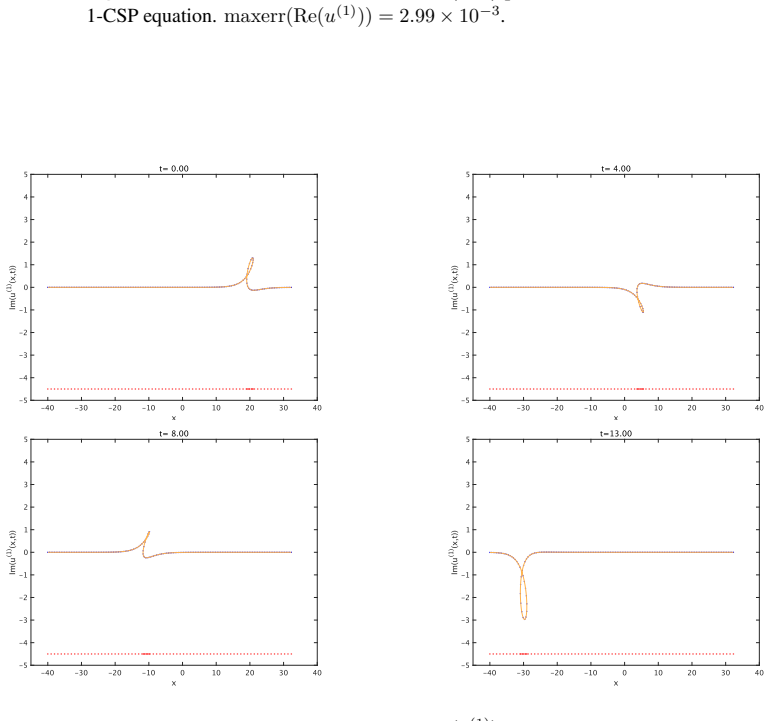
- Section 5: all accuracy claims rest on continuous exact one- and two-soliton initial data (and the corresponding continuous hodograph mesh). While the reported maxerr values are convincing for those families, the paper does not test non-soliton or multi-soliton (N>2) data, nor does it examine long-time stability under the adaptive mesh. A brief additional experiment or an explicit caveat that the observed accuracy is demonstrated only for the soliton families of Section 5 would keep the numerical claim proportionate to the evidence.
minor comments (5)
- Abstract and Introduction: the phrase “practical self-adaptive moving mesh scheme” is repeated; a single, precise statement would suffice.
- Equation (2.17) and subsequent Pfaffian elements: the condition that all denominators are nonzero is stated only once; a short global remark at the beginning of Section 2 would avoid later repetition.
- Figures 5.1–5.22: the captions report maxerr but do not indicate the final time T or the number of time steps; adding these data would make the error figures self-contained.
- References [33] and [37–38] are earlier works by overlapping authors on semi-discretizations; a one-sentence clarification of what is new relative to those papers would help the reader.
- Typographical: “sho rt” appears in the running title; “T wo-soliton” and similar line-break artifacts occur in several places (e.g., Examples 2.3, 4.5).
Circularity Check
No significant circularity: discrete equations and Pfaffian solutions are constructed independently; numerics only verify consistency.
full rationale
The paper's central claims rest on an explicit bilinear construction. Continuous MCSP is mapped via hodograph (2.3) and dependent-variable change (2.11) to bilinear system (2.12); Theorem 2.1 and Lemma 2.2 then exhibit Pfaffian N-soliton solutions by direct expansion and Pfaffian identities. Semi-discrete (3.1) and fully discrete (4.1) bilinear systems are postulated by the same method; Theorems 4.1–4.3 and Lemmas 3.1–3.2 verify that the same Pfaffian elements (with discrete exponential factors) satisfy them and that the dependent-variable map (4.25) produces the nonlinear difference equations (4.30). Continuous and semi-discrete limits are recovered by Taylor expansion (Remark 4.4). Numerical Section 5 initializes the scheme from the continuous exact solutions and reports peak relative errors; this is consistency checking, not a fitted prediction. Self-citations to earlier SP/CSP discretizations by overlapping authors supply background technique (hodograph + bilinear) but are not load-bearing for the new multi-component full discretization or its Pfaffian solutions. No parameter is fitted to data and then re-presented as a prediction; no uniqueness theorem is imported solely by self-citation to forbid alternatives. The derivation is therefore self-contained against its own algebraic benchmarks.
Axiom & Free-Parameter Ledger
free parameters (2)
- lattice spacings a, b =
a=0.005, b=0.0005
- soliton spectral and phase parameters (p_j, B_j, a_j^{(μ)}, b_k^{(ν)})
axioms (3)
- standard math Hirota D-operator bilinear calculus and the standard Pfaffian expansion identities (cited as [41]) hold for the introduced elements.
- domain assumption The continuous multi-component short-pulse equation (1.2) and its complex reduction (1.3) are the correct continuum models.
- ad hoc to paper All denominators appearing in the discrete equations and Pfaffian elements remain nonzero for the solutions under consideration.
invented entities (1)
-
Pfaffian multi-component short-pulse bilinear system (2.12) and its fully discrete analogue (4.1)/(4.30)
independent evidence
read the original abstract
We propose a new formulation of the multi-component short pulse (MCSP) equation that includes the coupled complex short pulse (CCSP) equation as a reduction. Using Hirota's bilinear method, we construct its $N$-soliton solutions in Pfaffian form. We then derive integrable semi-discrete and fully discrete analogues of the MCSP equation admitting Pfaffian $N$-soliton solutions. The resulting fully discrete system provides a practical self-adaptive moving mesh scheme for numerical simulations. For the parameter sets considered, numerical simulations demonstrate excellent agreement between the numerical and exact solutions, confirming the robustness and high accuracy of the proposed scheme.
Figures




Reference graph
Works this paper leans on
-
[1]
Hirota R 1977 Nonlinear partial difference equations. I. A difference analogue of the Korteweg-de Vries equation J. Phys. Soc. Jpn. 43 1424–1433
1977
-
[2]
Hirota R 1977 Nonlinear partial difference equations. I I . Discrete–time Toda equation J. Phys. Soc. Jpn. 43 2074–2078
1977
-
[3]
Hirota R 1977 Nonlinear partial difference equations. I I I. Discrete sine–Gordon equation J. Phys. Soc. Jpn. 43 2079–2086
1977
-
[4]
Hirota R 1978 Nonlinear partial difference equations. I V . B ¨acklund transformation for the discrete-time Toda equation J. Phys. Soc. Jpn. 45 321–332
1978
-
[5]
Hirota R 1979 Nonlinear partial difference equations. V . Nonlinear equations reducible to linear equations J. Phys. Soc. Jpn. 46 312–319 Integrable full discretization of the multi-component sho rt pulse equation 48
1979
-
[6]
Hirota R 1981 Discrete analogue of a generalized Toda equ ation J. Phys. Soc. Jpn. 50 3785–3791
1981
-
[7]
Ablowitz M J and Ladik J F 1975 Nonlinear differential-diff erence equations J. Math. Phys. 16 598–603
1975
-
[8]
Ablowitz M J and Ladik J F 1976 Nonlinear differential-diff erence equations and Fourier analysis J. Math. Phys. 17 1011–1018
1976
-
[9]
Ablowitz M J and Ladik J F 1976 A nonlinear difference schem e and inverse scattering Stud. Appl. Math. 55 213–229
1976
-
[10]
Ablowitz M J and Ladik J F 1977 On the solution of a class of nonlinear partial difference equations Stud. Appl. Math. 57 1–12
1977
-
[11]
Ablowitz M J and Segur H 1981 Solitons and the Inverse Scattering Transform (Philadelphia: Society for Industrial and Applied Mathematics)
1981
-
[12]
Suris Y B 2003 The Problem of Integrable Discretization: Hamiltonian App roach (Basel: Springer)
2003
-
[13]
Hietarinta J, Joshi N and Nijhoff F W 2016 Discrete Systems and Integrability (Cambridge: Cambridge University Press)
2016
-
[14]
Wadati M, Konno K and Ichikawa Y 1979 New integrable nonl inear evolution equations J. Phys. Soc. Jpn. 47 1698–1700
1979
-
[15]
Konno K, Ichikawa Y and Wadati M 1981 A loop soliton propa gating along a stretched rope J. Phys. Soc. Jpn. 50 1025–1026
1981
-
[16]
Ishimori Y 1981 On the modified Korteweg-de Vries solito n and the loop soliton J. Phys. Soc. Jpn. 50 2471–2472
1981
-
[17]
Ishimori Y 1982 A relationship between the Ablowitz-Ka up-Newell-Segur and Wadati-Konno-Ichikawa schemes of the inverse scattering method J. Phys. Soc. Jpn. 51 3036–3041
1982
-
[18]
Wadati M and Sogo K 1983 Gauge transformations in solito n theory J. Phys. Soc. Jpn. 52 394–398
1983
-
[19]
Rogers C and Schief W K 2002 B¨acklund and Darboux Transformations: Geometry and Modern Applications in Soliton Theory (Cambridge: Cambridge University Press)
2002
-
[20]
Feng B F, Maruno K and Ohta Y 2010 Integrable discretizat ions of the short pulse equation J. Phys. A: Math. Theor. 43 085203
2010
-
[21]
Feng B F, Inoguchi J, Kajiwara K, Maruno K and Ohta Y 2013 I ntegrable discretizations of the Dym equation Front. Math. China 8 1017–1029
2013
-
[22]
Feng B F, Maruno K and Ohta Y 2014 Self-adaptive moving me sh schemes for short pulse type equations and their Lax pairs Pac. J. Math. Ind. 6 1–14
2014
-
[23]
Ohta Y , Maruno K and Feng B F 2008 An integrable semi-disc retization of the Camassa-Holm equation and its determinant solution J. Phys. A: Math. Theor. 41 355205
2008
-
[24]
Feng B F, Maruno K and Ohta Y 2010 A self-adaptive moving mesh method for the Camassa-Holm equation J. Comput. Appl. Math. 235 229–243
2010
-
[25]
Feng B F, Maruno K and Ohta Y 2010 Integrable discretizat ions for the short-wave model of the Camassa- Holm equation J. Phys. A: Math. Theor. 43 265202
2010
-
[26]
Feng B F, Maruno K and Ohta Y 2015 Integrable semi-discre tizations of the reduced Ostrovsky equation J. Phys. A: Math. Theor. 48 135203
2015
-
[27]
Feng B F, Maruno K and Ohta Y 2017 An integrable semi-discrete Degasperis-Procesi equationNonlinearity 30 2246–2267
2017
-
[28]
Sch ¨afer T and Wayne C E 2004 Propagation of ultra-short optical p ulses in cubic nonlinear media Physica D 196 90–105
2004
-
[29]
Chung Y , Jones C K R T, Sch ¨afer T and Wayne C E 2005 Ultra-short pulses in linear and nonl inear media Nonlinearity 18 1351–1374
2005
-
[30]
Sakovich A and Sakovich S 2005 The short pulse equation i s integrable J. Phys. Soc. Jpn. 74 239–241
2005
-
[31]
Sakovich A and Sakovich S 2006 Solitary wave solutions o f the short pulse equation J. Phys. A: Math. Gen. 39 L361–L367
2006
-
[32]
Matsuno Y 2007 Multiloop soliton and multibreather sol utions of the short pulse model equation J. Phys. Soc. Jpn. 76 084003
2007
-
[33]
Hori A, Maruno K, Ohta Y and Feng B F 2025 Integrable self- adaptive moving mesh schemes for multi- component short pulse type equations with nonzero boundary values arXiv:2507.03880 Integrable full discretization of the multi-component sho rt pulse equation 49
Pith/arXiv arXiv 2025
-
[34]
Feng B F, Inoguchi J, Kajiwara K, Maruno K and Ohta Y 2011 D iscrete integrable systems and hodograph transformations arising from motions of discrete plane cur ves J. Phys. A: Math. Theor. 44 395201
2011
-
[35]
Matsuno Y 2011 A novel multi-component generalization of the short pulse equation and its multisoliton solutions J. Math. Phys. 52 123702
2011
-
[36]
Feng B F 2012 An integrable coupled short pulse equation J. Phys. A: Math. Theor. 45 085202
2012
-
[37]
Feng B F, Maruno K and Ohta Y 2015 Integrable semi-discre tization of a multi-component short pulse equation J. Math. Phys. 56 043502
2015
-
[38]
Feng B F, Chen J, Chen Y , Maruno K and Ohta Y 2015 Integrabl e discretizations and self-adaptive moving mesh method for a coupled short pulse equation J. Phys. A: Math. Theor. 48 385202
2015
-
[39]
Feng B F 2015 Complex short pulse and coupled complex sho rt pulse equations Physica D 297 62–75
2015
-
[40]
Hirota R 2000 Discretization of coupled modified KdV equ ations Chaos, Solitons & Fractals 11 77–84
2000
-
[41]
Hirota R 2004 The Direct Method in Soliton Theory (Cambridge: Cambridge University Press)
2004
discussion (0)
Sign in with ORCID, Apple, or X to comment. Anyone can read and Pith papers without signing in.