REVIEW 3 major objections 10 minor 55 references
Reviewed by Pith at T0; open to challenge.
T0 means a machine referee read the full paper against a public rubric. The mark states how deep the mechanical check went, never who wrote it. the ladder, T0–T4 →
T0 review · glm-5.2
Extragradient prediction step makes SAM less sensitive to its key knob
2026-07-08 14:58 UTC pith:3FCIOLPE
load-bearing objection EISAM combines extragradient prediction with SAM; experiments are broad but theory-experiment gap and Algorithm 1 discrepancy need resolution. the 3 major comments →
Leveraging Extragradient for Effective Sharpness-Aware Minimization in Deep Learning
The pith
A machine-rendered reading of the paper's core claim, the machinery that carries it, and where it could break.
Core claim
The central mechanism is the prediction step y_t = w_t − s∇F(w_t), which probes the loss landscape geometry before the SAM perturbation is applied. Under strong-convexity and smoothness assumptions, this step introduces a (1−sμ)² factor into the generalization bound's denominator (tightening it relative to SAM's bound of 1) while relegating the perturbation radius ρ to higher-order error terms. This structural separation—prediction step sharpens the bound, ρ only affects residuals—is what the authors identify as the source of reduced ρ-sensitivity. The nonconvex extension (Theorem 4) shows s and ρ entering a shared denominator factor (1−sL−ρL) with a direct variance trade-off, but the key (1
What carries the argument
Extragradient-inspired prediction step (Eq. 4–5): y_t = w_t − s∇F_S(w_t), followed by SAM perturbation at y_t and gradient update from the perturbed point. The (1−sμ)² tightening factor in the generalization bound arises from co-coercivity applied to the trajectory difference between two datasets differing by one sample.
Load-bearing premise
The theoretical tightening of the generalization bound by (1−sμ)² is derived under μ-strong convexity and L-smoothness of the loss function, assumptions that do not hold for deep neural network loss landscapes where the experiments are conducted. The nonconvex extension invokes a local Polyak–Łojasiewicz inequality without justification, and its bound structure differs from the convex analysis used to motivate the tightening claim.
What would settle it
If sweeping ρ across a wide range for EISAM on a large-scale task (e.g., ImageNet with ViT) shows the same accuracy variance as standard SAM, the reduced-sensitivity claim would be empirically falsified.
If this is right
- If the (1−sμ)² tightening carries over to practical nonconvex settings, EISAM could reduce the hyperparameter tuning burden for SAM-family optimizers, which currently require careful per-task ρ selection.
- The prediction-step idea could be composed with other SAM variants (ASAM, GSAM, FSAM) to further reduce their ρ-sensitivity, since the mechanism is orthogonal to how the perturbation direction is chosen.
- If reduced ρ-sensitivity holds at scale, it could lower the cost of hyperparameter search for sharpness-aware training of large models, where grid searches over ρ are expensive.
Editorial analysis
A structured set of objections, weighed in public.
Referee Report
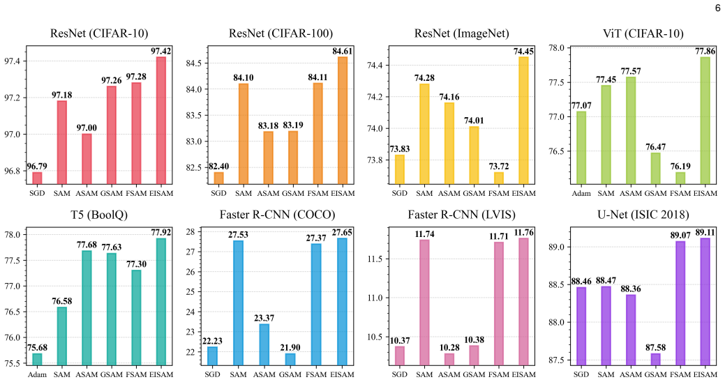
Summary. The paper proposes EISAM, an optimizer that augments Sharpness-Aware Minimization (SAM) with an extragradient-inspired prediction step. The method computes an intermediate point via a gradient step, then evaluates the SAM perturbation at that point. Theoretical analysis under strong convexity claims that the prediction step tightens the generalization bound by a factor of (1-sμ)^2 in the denominator relative to SAM, and that the perturbation radius ρ only affects higher-order terms. Experiments span image classification (CIFAR-10/100, ImageNet-1K), NLP (BOOLQ), object detection (COCO, LVIS), and segmentation (ISIC2018), comparing against SGD, Adam, SAM, ASAM, GSAM, and FSAM. The breadth of experiments and the hyperparameter sensitivity analysis are commendable. However, a critical disconnect exists between the algorithm as written (Algorithm 1) and both the theoretical analysis and the mathematical formulation (Eq. 5), which must be resolved.
Significance. The paper provides a falsifiable theoretical claim (the (1-sμ)^2 tightening and ρ-only-higher-order claim) and tests it across a diverse set of tasks and architectures. The hyperparameter sensitivity analysis (Fig. 7-9) directly addresses the practical concern of ρ-tuning in SAM. The computational cost comparison (Table 9) is a useful addition. The Hessian spectra analysis (Fig. 4) provides empirical evidence connecting the method to flat minima. These are genuine strengths. However, the significance is substantially undermined by the algorithm-theory disconnect described below.
major comments (3)
- Algorithm 1 (§3.3) does not apply the perturbation ε before the sharpness-aware gradient evaluation. Line 5 computes ε = ρ·g/||g||, but line 6 computes g_sam = ∇F_B(w) where w = y_t (set on line 4), with no addition of ε. Line 7's opt.update(w, g_sam, η) receives no ε argument. This means Algorithm 1 implements plain extragradient (predict at y_t, evaluate gradient at y_t), not sharpness-aware minimization at a perturbed point. This directly contradicts Eq. (5), which specifies w_{t+1} = y_t - η∇F_S(y_t + ε_t), and the three-step update in §4.1 (steps 2-3), which analyzes ∇F_{B_t}(w'_t) where w'_t = y_t + ε_t. The theoretical analysis (Lemmas 1-3, Theorems 1-3) all depend on the perturbed-point version. If Algorithm 1 reflects the actual code, then ρ should have zero effect on the algorithm, yet Fig. 7 shows clear ρ-sensitivity, suggesting the code does something not captured by the psud
- §4.5, Theorem 4: The nonconvex extension invokes a local Polyak-Łojasiewicz (PL) inequality in the proof (Appendix B.7) without stating it as an assumption in Theorem 4's conditions or Definition 5. The PL inequality is a strong structural assumption that is not standard for deep neural network loss landscapes and is not justified empirically. Since the convex analysis (Theorems 1-3) does not apply to the experimental setting (deep networks are non-convex), Theorem 4 is the only theoretical result potentially applicable to the experiments, making this unjustified assumption load-bearing for the claim that the theory supports the empirical results.
- §4.4, Theorem 3: The claim that the generalization bound is 'tightened' by (1-sμ)^2 relative to standard SAM is a direct algebraic consequence of the prediction step's effect on the trajectory difference δ_t (Lemma 1). The factor (1-sμ)^2 arises because the prediction step y_t = w_t - s∇F(w_t) shrinks the inter-trajectory distance by (1-sμ) under strong convexity. This is not an independent tightening mechanism but rather a restatement of the contraction property. The paper should clarify that this is an algebraic consequence of the prediction step's contraction, not a separate sharpness-aware improvement, and should note that the same factor would appear for any prediction-step method (e.g., plain extragradient without the SAM perturbation).
minor comments (10)
- §3.3: The text states 'EISAM approximates it using ∇F_S(w_t) for efficiency, actually simulates three gradient computations.' This sentence is grammatically incomplete and unclear.
- §3.3, Algorithm 1, Line 4: 'update parameters w ← y' is ambiguous — it is unclear whether this is a permanent update or a temporary reassignment for the purpose of the subsequent gradient computation. This should be clarified.
- §3.4: 'EISAM displays a hign peak early on' — typo: 'hign' should be 'high'.
- §5.2: The text refers to 'AdamW achieved solid performance' but Table 5 lists 'Adam' as the optimizer. This inconsistency should be resolved.
- §5.1: The text states 'no data augmentation was used' on ImageNet-1K 'to maintain experimental consistency,' but CutMix was used on CIFAR. This is inconsistent and the rationale is unclear.
- Table 4: GSAM and FSAM show notably poor performance on ViT-S-8(Cutmix) and ViT-S-16(Cutmix) compared to SAM. This is unusual and warrants brief discussion.
- Fig. 9 caption: 'The elliptical contour plot in Fig. 9 is centered at the origin' — it is unclear what 'centered at the origin' means in this context (origin of what axes?).
- Appendix B.1: The proof states 'After computing y_t, we update w_t ← y_t, and the perturbation uses the initial gradient at the original w_t.' This is inconsistent with Eq. (5) and §4.1, which state the perturbation uses ∇F_S(y_t). The paper should clarify which gradient is used for the perturbation direction.
- Table 10: EISAM-s values vary across settings (5e-3, 1e-3, 1e-4, 5e-4). The text states 'for most tasks, directly adopting the default values... is sufficient,' but the table shows substantial variation. This should be reconciled.
- §4.1: The three-step update description (steps 1-3) uses w'_t = y_t + ρ∇F_{B_t}(w_t)/||∇F_{B_t}(w_t)||, but Eq. (5) and §3.3 use ε_t = ρ∇F_S(y_t)/||∇F_S(y_t)|| (or the approximation using w_t). The perturbation direction is inconsistent between §3.3 and §4.1.
Simulated Author's Rebuttal
We thank the referee for a careful reading and for identifying a genuine inconsistency in Algorithm 1. We address each comment below and commit to revisions where the referee is correct.
read point-by-point responses
-
Referee: Algorithm 1 does not apply the perturbation ε before the sharpness-aware gradient evaluation. Line 5 computes ε but line 6 computes g_sam = ∇F_B(w) at y_t without adding ε. This contradicts Eq. (5) and the analysis in §4.1. If Algorithm 1 reflects the actual code, ρ should have zero effect, yet Fig. 7 shows ρ-sensitivity.
Authors: The referee is correct that Algorithm 1 as written contains an error: it does not add ε to the parameters before computing the sharpness-aware gradient, contradicting Eq. (5) and the theoretical analysis in §4.1. The intended algorithm—and the one actually implemented in our code—is: (1) compute g = ∇F_B(w_t); (2) compute the prediction point y_t = w_t - s·g and set w ← y_t; (3) compute ε = ρ·g/||g||; (4) compute g_sam = ∇F_B(w + ε); (5) update w via the base optimizer using g_sam. The perturbation ε is applied to the current parameters (which equal y_t after line 4) before the gradient evaluation. This is consistent with Eq. (5), the three-step update in §4.1, and all theoretical results. The ρ-sensitivity in Fig. 7 confirms that the implementation does apply the perturbation. We will correct Algorithm 1 to explicitly show the addition w ← w + ε before computing g_sam, ensuring the pseudocode matches Eq. (5) and the proofs. We will also add a clarifying remark that the gradient used for the perturbation direction is the gradient at the original w_t (before the prediction step), as noted in the text of §3.3 and in the proof of Lemma 1 (Appendix B.1: 'the perturbation uses the initial gradient at the original w_t'). revision: yes
-
Referee: Theorem 4 invokes a local Polyak-Łojasiewicz (PL) inequality in the proof (Appendix B.7) without stating it as an assumption in Theorem 4's conditions or Definition 5. The PL inequality is a strong structural assumption not standard for deep neural network loss landscapes and is not justified empirically. Since Theorem 4 is the only result potentially applicable to the experiments, this unjustified assumption is load-bearing.
Authors: The referee is correct that the local PL inequality is used in the proof of Theorem 4 (Appendix B.7) but is not stated as an assumption in Theorem 4's conditions or in Definition 5. This is an omission in the manuscript. We will add the local PL inequality as an explicit assumption in the statement of Theorem 4 and in Definition 5. We also acknowledge the referee's point that the PL condition is a strong structural assumption that is not standard for deep neural network loss landscapes and is not justified empirically in our paper. We will add a candid discussion of this limitation: the nonconvex result should be understood as applying under the PL condition (which holds in certain structured settings such as over-parameterized models near global minima, as studied by Liu et al. 2022 and others), and the connection to our experimental results is therefore motivational rather than a direct theoretical guarantee. We will also note that the convex results (Theorems 1–3) provide the core theoretical insight—that the prediction step introduces the (1-sμ)^2 contraction factor—while Theorem 4 extends the analysis to a nonconvex setting under additional structural assumptions. We do not claim that Theorem 4 directly applies to deep networks without the PL assumption. revision: yes
-
Referee: The (1-sμ)^2 tightening relative to SAM is a direct algebraic consequence of the prediction step's contraction property, not an independent sharpness-aware improvement. The same factor would appear for any prediction-step method (e.g., plain extragradient without the SAM perturbation). The paper should clarify this.
Authors: The referee's mathematical observation is correct: the (1-sμ)^2 factor arises from the contraction property of the prediction step under strong convexity, and it would appear for any prediction-step method that moves to y_t = w_t - s∇F(w_t) before evaluating the gradient. We agree that the paper should clarify this. We will revise the presentation to explicitly state that the tightening is an algebraic consequence of the prediction step's contraction, not a separate sharpness-aware mechanism. However, we wish to note that the key contribution is not the factor in isolation but rather the observation that combining the prediction step with the SAM perturbation yields a bound where ρ appears only in higher-order terms (Theorem 3), which is a property specific to the EISAM construction and not shared by plain extragradient without the SAM perturbation. The prediction step changes the point at which the SAM perturbation is evaluated, and the interaction between the contraction and the perturbation structure is what produces the reduced ρ-sensitivity in the bound. We will make this distinction clear in the revised manuscript. revision: partial
Circularity Check
No significant circularity: the (1-sμ)² tightening is an algebraic consequence of the prediction-step ansatz, not a fit-to-prediction loop or self-citation chain.
full rationale
The paper's central theoretical claim is that EISAM tightens the generalization bound by a factor of (1-sμ)² in the denominator relative to SAM (Theorem 3, §4.4). Walking the derivation chain: the prediction step y_t = w_t - s∇F(w_t) (Eq. 4) introduces the factor (1-sμ) through the identity (I - sH_t) acting on the trajectory difference δ_t (Lemma 1, Appendix B.1). The co-coercivity lemma (citing Hardt et al. [50], an external reference) then produces the contraction factor (1-sμ)² in the stability bound. This is a direct algebraic consequence of the algorithm's definition, not a fitted parameter renamed as a prediction. The paper does not fit s to the generalization bound and then claim to predict it. The ρ-only-affects-higher-order-terms claim similarly follows from the Taylor expansion structure where ρ enters via the perturbation w'_t = y_t + ρ∇F/||∇F|| and contributes O(ρδ²/G) terms that are higher-order relative to the leading (1-sμ)²δ² term. While the skeptic correctly notes a disconnect between Algorithm 1 (which does not apply ε before computing g_sam) and the theoretical analysis (which analyzes the perturbed-point version), this is a correctness/consistency issue, not circularity. The theoretical analysis is self-contained: assumptions (strong convexity, smoothness, Lipschitz) are standard, the key tool (co-coercivity) is externally cited, and no self-citation chain is load-bearing. The nonconvex extension (Theorem 4) invokes a local Polyak-Łojasiewicz inequality without justification, but this is an unsupported-assumption concern, not circularity. No step in the derivation reduces to its inputs by construction in the sense of the circularity patterns enumerated.
Axiom & Free-Parameter Ledger
free parameters (4)
- ρ (perturbation radius) =
0.001-0.2 (task-dependent)
- s (prediction step size) =
1e-5 to 0.01 (default 1e-3)
- η (learning rate) =
0.01-0.1 (vision), 1e-4 to 5e-4 (NLP)
- weight decay =
1e-5 to 2e-3
axioms (5)
- domain assumption Loss function is μ-strongly convex (Definition 1, §4.1)
- domain assumption Loss function is L-smooth (Definition 2, §4.1)
- domain assumption Loss function is G-Lipschitz continuous (Definition 3, §4.1)
- domain assumption Hessian is K-Lipschitz continuous with bounded remainder (Definition 4, §4.1)
- ad hoc to paper Local Polyak-Łojasiewicz inequality (§4.5, Theorem 4 proof)
read the original abstract
Generalization remains a pivotal challenge in deep learning, where traditional optimizers like Stochastic Gradient Descent (SGD) often converge to sharp minima, leading to overfitting and reduced performance on unseen data. Building on Sharpness-Aware Minimization (SAM), for seeking flat minima associated with improved generalization, we propose the Extragradient-Inspired Sharpness-Aware Minimization (EISAM), a novel optimizer that enhances generalization via the extragradient technique. EISAM uses a two-step update process: a prediction step investigating the geometry of the loss landscape and a perturbation step that refines updates with a base optimizer. This approach achieves better generalization performance than SAM. Crucially, EISAM reduces sensitivity to the perturbation radius, enhancing robustness, and simplifying the tuning across diverse settings. Extensive experiments on benchmark datasets demonstrate that EISAM consistently outperforms SGD, Adaptive Moment Estimation (Adam), and SAM in test accuracy and training efficiency across various architectures. Theoretical analysis further confirms that EISAM tightens the generalization bound by steering parameters toward flatter minima with reduced curvature. Accompanied by a thorough hyperparameter analysis, EISAM offers practical tuning guidance, establishing it as a robust, scalable, and broadly applicable optimization solution that advances both the theory and practice in deep learning.
Figures


Reference graph
Works this paper leans on
-
[1]
Sharp minima can generalize for deep nets,
L. Dinh, R. Pascanu, S. Bengio, and Y. Bengio, “Sharp minima can generalize for deep nets,” inProc. Int. Conf. Mach. Learn., 2017, pp. 1019–1028
work page 2017
-
[2]
S. Hochreiter and J. Schmidhuber, “Flat minima,”Neural Computa- tion, vol. 9, no. 1, pp. 1–42, 1997
work page 1997
-
[3]
On large-batch training for deep learning: Generalization gap and sharp minima,
N. S. Keskar, D. Mudigere, J. Nocedal, M. Smelyanskiy, and P . T. P . Tang, “On large-batch training for deep learning: Generalization gap and sharp minima,” inProc. Int. Conf. Learn. Represent., 2017
work page 2017
-
[4]
Sharpness- aware minimization for efficiently improving generalization,
P . Foret, A. Kleiner, H. Mobahi, and B. Neyshabur, “Sharpness- aware minimization for efficiently improving generalization,” in Proc. Int. Conf. Learn. Represent., 2021
work page 2021
-
[5]
Extragra- dient method in optimization: Convergence and complexity,
T. P . Nguyen, E. Pauwels, ´E. Richard, and B. W. Suter, “Extragra- dient method in optimization: Convergence and complexity,”J. Optim. Theory Appl., vol. 176, no. 1, pp. 137–162, 2018
work page 2018
-
[6]
Learning multiple layers of features from tiny images,
A. Krizhevsky, “Learning multiple layers of features from tiny images,” University of Toronto, Tech. Rep. Tech. Rep. TR-2009, 2009
work page 2009
-
[7]
ImageNet: a large-scale hierarchical image database,
J. Deng, W. Dong, R. Socher, L.-J. Li, K. Li, and L. Fei-Fei, “ImageNet: a large-scale hierarchical image database,”Proc. IEEE, vol. 97, no. 11, pp. 248–255, 2009
work page 2009
-
[8]
Microsoft COCO: common objects in context,
T.-Y. Lin, M. Maire, S. Belongie, J. Hays, P . Perona, D. Ramanan, P . Doll´ar, and C. L. Zitnick, “Microsoft COCO: common objects in context,” inComputer Vision – ECCV 2014, ser. Lecture Notes in Computer Science, vol. 8693, 2014, pp. 740–755
work page 2014
-
[9]
LVIS: A dataset for large vo- cabulary instance segmentation,
A. Gupta, P . Doll ´ar, and R. Girshick, “LVIS: A dataset for large vo- cabulary instance segmentation,” inProc. IEEE/CVF Conf. Comput. Vis. Pattern Recognit. (CVPR), 2019
work page 2019
-
[10]
N. Codella, V . Rotemberg, P . Tschandl, M. E. Celebi, S. Dusza, D. Gutman, B. Helba, A. Kalloo, K. Liopyris, M. Marchetti, H. Kittler, and A. Halpern, “Skin lesion analysis toward melanoma detection 2018: A challenge hosted by the international skin imaging collaboration (ISIC),” 2019. [Online]. Available: https://arxiv.org/abs/1902.03368
work page internal anchor Pith review Pith/arXiv arXiv 2018
-
[11]
BoolQ: exploring the surprising difficulty of natu- ral yes/no questions,
C. Clark, K. Lee, M.-W. Chang, T. Kwiatkowski, M. Collins, and K. Toutanova, “BoolQ: exploring the surprising difficulty of natu- ral yes/no questions,”Trans. Assoc. Comput. Linguistics, vol. 7, pp. 2924–2943, 2019
work page 2019
-
[12]
Towards understanding sharpness-aware minimization,
M. Andriushchenko and N. Flammarion, “Towards understanding sharpness-aware minimization,” inProc. Int. Conf. Mach. Learn., ser. Proc. Mach. Learn. Res., vol. 162, 2022, pp. 639–668
work page 2022
-
[13]
Entropy-SGD: Biasing gradient descent into wide valleys,
P . Chaudhari, A. Choromanska, S. Soatto, Y. LeCun, C. Baldassi, C. Borgs, J. Chayes, L. Sagun, and R. Zecchina, “Entropy-SGD: Biasing gradient descent into wide valleys,” inProc. Int. Conf. Learn. Represent. (ICLR), 2017
work page 2017
-
[14]
Visualizing the loss landscape of neural nets,
H. Li, Z. Xu, G. Taylor, C. Studer, and T. Goldstein, “Visualizing the loss landscape of neural nets,” inProc. Adv. Neural Inf. Process. Syst., vol. 31, 2018, pp. 6391–6401
work page 2018
-
[15]
A modern look at the relationship between sharpness and generalization,
M. Andriushchenko, F. Croce, M. M ¨uller, M. Hein, and N. Flam- marion, “A modern look at the relationship between sharpness and generalization,” inProc. Int. Conf. Mach. Learn. (ICML), 2023
work page 2023
-
[16]
Flat minima and generalization: Insights from stochastic convex optimization,
M. Schliserman, S. Vansover-Hager, and T. Koren, “Flat minima and generalization: Insights from stochastic convex optimization,”
-
[17]
Flat Minima and Generalization: Insights from Stochastic Convex Optimization
[Online]. Available: https://arxiv.org/abs/2511.03548
work page internal anchor Pith review Pith/arXiv arXiv
-
[18]
The Split Matters: Flat Minima Methods for Improving the Performance of GNNs
N. Lell and A. Scherp, “The split matters: Flat minima methods for improving the performance of gnns,” 2023. [Online]. Available: https://arxiv.org/abs/2306.09121
work page internal anchor Pith review Pith/arXiv arXiv 2023
-
[19]
Do sharpness- based optimizers improve generalization in medical image analy- sis?
M. Hassan, A. Vakanski, B. Zhang, and M. Xian, “Do sharpness- based optimizers improve generalization in medical image analy- sis?”IEEE Access, vol. 13, pp. 82 972–82 985, 2025
work page 2025
-
[20]
ASAM: Adaptive sharpness-aware minimization for scale-invariant learning of deep neural networks,
J. Kwon, J. Kim, H. Park, and I.-K. Choi, “ASAM: Adaptive sharpness-aware minimization for scale-invariant learning of deep neural networks,” inProc. Int. Conf. Mach. Learn., ser. Proc. Mach. Learn. Res., vol. 139, 2021, pp. 5905–5914
work page 2021
-
[21]
Sharpness-aware lookahead for accelerating convergence and improving generalization,
C. Tan, J. Zhang, J. Liu, and Y. Gong, “Sharpness-aware lookahead for accelerating convergence and improving generalization,”IEEE Trans. Pattern Anal. Mach. Intell., vol. 46, no. 12, pp. 10 375–10 388, 2024
work page 2024
-
[22]
Query-efficient meta attack to deep neural networks,
J. Du, H. Zhang, J. T. Zhou, Y. Yang, and J. Feng, “Query-efficient meta attack to deep neural networks,” inProc. Int. Conf. Learn. Represent. (ICLR), 2020
work page 2020
-
[23]
Friendly sharpness-aware minimization,
T. Li, P . Zhou, Z. He, X. Cheng, and X. Huang, “Friendly sharpness-aware minimization,” inProc. IEEE/CVF Conf. Comput. Vis. Pattern Recognit. (CVPR), 2024
work page 2024
-
[24]
Surrogate gap minimiza- tion improves sharpness-aware training,
J. Zhuang, B. Gong, L. Yuan, Y. Cui, H. Adam, N. Dvornek, S. Tatikonda, and T. L. James Duncan, “Surrogate gap minimiza- tion improves sharpness-aware training,” inProc. Int. Conf. Learn. Represent. (ICLR), 2022
work page 2022
-
[25]
Sharpness-aware minimization: General analysis and improved rates,
D. Oikonomou and N. Loizou, “Sharpness-aware minimization: General analysis and improved rates,” inProc. Int. Conf. Learn. Represent. (ICLR), 2025
work page 2025
-
[26]
A method for solving the convex programming problem with convergence rateO(1/k 2),
Y. Nesterov, “A method for solving the convex programming problem with convergence rateO(1/k 2),”Dokl. Akad. Nauk SSSR, vol. 269, no. 3, pp. 543–547, 1983
work page 1983
-
[27]
From error bounds to the complexity of first-order descent methods for convex functions,
J. Bolte, T. P . Nguyen, J. Peypouquet, and B. W. Suter, “From error bounds to the complexity of first-order descent methods for convex functions,”Math. Program., vol. 165, no. 2, pp. 471–507, 2017. 16
work page 2017
-
[28]
D. A. McAllester, “PAC-bayesian model averaging,” inProc. 12th Annu. Conf. Comput. Learn. Theory. ACM Press, 1999, pp. 164–170
work page 1999
-
[29]
Fantastic generalization measures and where to find them,
Y. Jiang, B. Neyshabur, H. Mobahi, D. Krishnan, and S. Bengio, “Fantastic generalization measures and where to find them,” in Proc. Int. Conf. Learn. Represent. (ICLR), 2020
work page 2020
-
[30]
Deep residual learning for image recognition,
K. He, X. Zhang, S. Ren, and J. Sun, “Deep residual learning for image recognition,” inProc. IEEE Conf. Comput. Vis. Pattern Recognit. (CVPR), 2016, pp. 770–778
work page 2016
-
[31]
Deep pyramidal residual networks,
D. Han, J. Kim, and J. Kim, “Deep pyramidal residual networks,” inProc. IEEE Conf. Comput. Vis. Pattern Recognit. (CVPR), 2017, pp. 6307–6315
work page 2017
-
[32]
S. Zagoruyko and N. Komodakis, “Wide residual networks,” in Proc. Brit. Mach. Vis. Conf., 2016
work page 2016
-
[33]
AutoAugment: Learning augmentation strategies from data,
E. D. Cubuk, B. Zoph, D. Mane, V . Vasudevan, and Q. V . Le, “AutoAugment: Learning augmentation strategies from data,” in Proc. IEEE/CVF Conf. Comput. Vis. Pattern Recognit. (CVPR), 2019, pp. 113–123
work page 2019
-
[34]
CutMix: Regularization strategy to train strong classifiers with localizable features,
S. Yun, D. Han, S. J. Oh, S. Chun, J. Choe, and Y. Yoo, “CutMix: Regularization strategy to train strong classifiers with localizable features,” inProc. IEEE/CVF Int. Conf. Comput. Vis. (ICCV), 2019, pp. 6023–6032
work page 2019
-
[35]
When does label smoothing help?
R. M ¨uller, S. Kornblith, and G. E. Hinton, “When does label smoothing help?” inProc. Adv. Neural Inf. Process. Syst., 2019
work page 2019
-
[36]
mixup: Beyond empirical risk minimization,
H. Zhang, M. Cisse, Y. N. Dauphin, and D. Lopez-Paz, “mixup: Beyond empirical risk minimization,” inProc. Int. Conf. Learn. Represent. (ICLR), 2018
work page 2018
-
[37]
Adam: A method for stochastic optimiza- tion,
D. P . Kingma and J. Ba, “Adam: A method for stochastic optimiza- tion,” inProc. Int. Conf. Learn. Represent. (ICLR), 2015
work page 2015
-
[38]
SGDR: Stochastic gradient descent with warm restarts,
I. Loshchilov and F. Hutter, “SGDR: Stochastic gradient descent with warm restarts,” inProc. Int. Conf. Learn. Represent. (ICLR), 2017
work page 2017
-
[39]
Lookahead optimizer: k steps forward, 1 step back,
M. R. Zhang, J. Lucas, J. Ba, and G. Hinton, “Lookahead optimizer: k steps forward, 1 step back,” inProc. Adv. Neural Inf. Process. Syst. (NeurIPS), 2019
work page 2019
-
[40]
RADAM: Texture recognition through randomized aggregated encoding of deep activation maps,
L. Scabini, K. M. Zielinski, L. C. Ribas, W. N. Gonc ¸alves, B. De Baets, and O. M. Bruno, “RADAM: Texture recognition through randomized aggregated encoding of deep activation maps,”Pattern Recognit., vol. 143, p. 109802, 2023
work page 2023
-
[41]
An automatic method for finding the greatest or least value of a function,
H. Rosenbrock, “An automatic method for finding the greatest or least value of a function,”Comput. J., vol. 3, pp. 175–184, 1960
work page 1960
-
[42]
The extragradient method for finding saddle points and other problems,
G. M. Korpelevich, “The extragradient method for finding saddle points and other problems,”Math. Notes (English Transl. of Matem- aticheskii Sbornik), vol. 12, pp. 747–756, 1976
work page 1976
-
[43]
Error bounds and convergence analysis of feasible descent methods: A general approach,
Z.-Q. Luo and P . Tseng, “Error bounds and convergence analysis of feasible descent methods: A general approach,”Ann. Oper. Res., vol. 46, no. 1, pp. 157–178, 1993
work page 1993
-
[44]
On the convergence of the proximal algorithm for nonsmooth functions involving analytic features,
H. Attouch and J. Bolte, “On the convergence of the proximal algorithm for nonsmooth functions involving analytic features,” Math. Program., vol. 116, no. 1, pp. 5–16, 2009
work page 2009
-
[45]
H. Attouch, J. Bolte, and B. F. Svaiter, “Convergence of descent methods for semi-algebraic and tame problems: Proximal algo- rithms, forward–backward splitting, and regularized gauss–seidel methods,”Math. Program., vol. 137, no. 1-2, pp. 91–129, 2013
work page 2013
-
[46]
Proximal alternating lin- earized minimization for nonconvex and nonsmooth problems,
J. Bolte, S. Sabach, and M. Teboulle, “Proximal alternating lin- earized minimization for nonconvex and nonsmooth problems,” Math. Program., vol. 146, no. 1-2, pp. 459–494, 2014
work page 2014
-
[47]
A fast iterative shrinkage-thresholding algorithm for linear inverse problems,
A. Beck and M. Teboulle, “A fast iterative shrinkage-thresholding algorithm for linear inverse problems,”SIAM J. Imaging Sci., vol. 2, no. 1, pp. 183–202, 2009
work page 2009
-
[48]
R. Zhou, M. Fazel, and S. S. Du, “Extragradient preference opti- mization (EGPO): Beyond last-iterate convergence for nash learn- ing from human feedback,” inProc. Conf. Lang. Model. (COLM), 2025
work page 2025
-
[49]
An investigation into neural net optimization via hessian eigenvalue density,
B. Ghorbani, S. Krishnan, and Y. Xiao, “An investigation into neural net optimization via hessian eigenvalue density,” inProc. Int. Conf. Mach. Learn. (ICML), vol. 97, 2019, pp. 2232–2241
work page 2019
-
[50]
O. Bousquet and A. Elisseeff, “Stability and generalization,”J. Mach. Learn. Res., vol. 2, pp. 499–526, 2002
work page 2002
-
[51]
Train faster, generalize better: Stability of stochastic gradient descent,
M. Hardt, B. Recht, and Y. Singer, “Train faster, generalize better: Stability of stochastic gradient descent,” inProc. Int. Conf. Mach. Learn. (ICML), 2016
work page 2016
-
[52]
An image is worth 16x16 words: Transformers for image recognition at scale,
A. Dosovitskiy, L. Beyer, A. Kolesnikov, D. Weissenborn, X. Zhai, T. Unterthiner, M. Dehghani, M. Minderer, G. Heigold, S. Gelly, J. Uszkoreit, and N. Houlsby, “An image is worth 16x16 words: Transformers for image recognition at scale,” inProc. Int. Conf. Learn. Represent. (ICLR), 2021
work page 2021
-
[53]
Faster R-CNN: Towards real-time object detection with region proposal networks,
S. Ren, K. He, R. Girshick, and J. Sun, “Faster R-CNN: Towards real-time object detection with region proposal networks,” inProc. Adv. Neural Inf. Process. Syst. (NeurIPS), vol. 28, 2015
work page 2015
-
[54]
U-Net: Convolutional networks for biomedical image segmentation,
O. Ronneberger, P . Fischer, and T. Brox, “U-Net: Convolutional networks for biomedical image segmentation,” inInt. Conf. Med. Image Comput. Comput.-Assist. Interv. (MICCAI), 2015, pp. 234–241
work page 2015
-
[55]
Exploring the limits of transfer learning with a unified text-to-text transformer,
C. Raffel, N. Shazeer, A. Roberts, K. Lee, S. Narang, M. Matena, Y. Zhou, W. Li, and P . J. Liu, “Exploring the limits of transfer learning with a unified text-to-text transformer,”J. Mach. Learn. Res., vol. 21, no. 140, pp. 1–67, 2020. Yao Fureceived the Master degree in Proba- bility and Statistics from Northeastern Univer- sity, Shenyang, China, in 201...
discussion (0)
Sign in with ORCID, Apple, or X to comment. Anyone can read and Pith papers without signing in.