REVIEW 3 major objections 6 minor 25 references
Sparse graphs beat dense ones for image classification
Reviewed by Pith at T0; open to challenge. T0 means a machine referee read the full paper against a public rubric. the ladder, T0–T4 →
T0 review · glm-5.2
2026-07-08 10:33 UTC pith:WMUUVFWY
load-bearing objection Honest empirical comparison of graph construction choices for GNN image classification, but a key design decision (randomized edge weights) may confound the central sparsity finding. the 3 major comments →
Visual graphs for image classification: does the structure affect performance?
The pith
A machine-rendered reading of the paper's core claim, the machinery that carries it, and where it could break.
Core claim
The paper demonstrates that aggressive graph sparsification, specifically reducing a graph to its minimum spanning tree, is the single most reliable route to strong classification performance across different node placement strategies and feature extractors. Eight of nine best-performing configurations use some form of pruning over the base dense graph, and six of nine use the most extreme pruning. The author interprets this as evidence that preserving only the strongest structural relationships, rather than maximizing connectivity, is what enables effective graph-based image classification.
What carries the argument
The experimental pipeline has three parametric dimensions: node extraction method (GRID at 7x7, SLIC superpixels, or Harris interest points), feature type (768-dim ViT, 256-dim CNN, or 130-dim SIFT), and graph model (base 6-NN, low-distance-mean pruning, locality-sensitive pruning, or MinCONN minimum spanning tree). The GCN itself is fixed at three layers with ReLU activations, global mean pooling, and softmax, so all performance variation is attributable to graph construction choices upstream of the network.
Load-bearing premise
The central claim rests on experiments conducted solely on Fashion-MNIST, a 28x28 grayscale dataset with 10 classes, using a single fixed GCN architecture with 50 nodes. The author acknowledges this limitation. The approximately 4 percent performance variation attributed to graph topology could be specific to this dataset's simplicity and may not hold on more complex, higher-resolution, or color imagery.
What would settle it
If running the same experimental matrix on a richer dataset (e.g., CIFAR-10 or ImageNet) with a deeper GCN shows that dense base graphs match or outperform MinCONN-pruned graphs, the core claim that sparsity is superior would not generalize.
If this is right
- If the finding generalizes, practitioners deploying graph neural networks on resource-constrained devices can use minimum spanning tree pruning to reduce edge counts dramatically without sacrificing, and potentially improving, classification accuracy.
- The result that richer node features (ViT at 768 dimensions) pair best with the sparsest graphs suggests an interaction between feature quality and topology: strong features may need less structural redundancy to propagate effectively.
- Graph construction pipelines for vision tasks could be simplified by defaulting to tree-structured graphs, reducing the design space from a continuum of density choices to a binary keep-or-prune decision.
Editorial analysis
A structured set of objections, weighed in public.
Referee Report
Summary. This paper presents an empirical study comparing different graph construction techniques (node extraction methods, feature types, and edge sparsification strategies) for image classification using a fixed three-layer GCN on Fashion-MNIST. The authors vary three dimensions: node extraction (grid, superpixel, interest points), feature descriptors (ViT, CNN, SIFT), and graph sparsification (base 6-NN, LDM, LSP, MinCONN/MST). The central claim is that graph architecture is not a neutral design choice, and that sparse graphs (particularly MinCONN) can achieve strong performance, suggesting that 'graph simplicity and structural quality are more critical than connectivity quantity.' The experimental protocol uses 10-fold stratified cross-validation with early stopping and a held-out test set, which is methodologically appropriate.
Significance. The paper addresses a practically relevant question for the graph-based vision community: how do graph construction choices affect GCN classification performance? The systematic comparison of node extraction, feature type, and sparsification within a controlled architecture is a useful methodological contribution. The experimental protocol (10-fold CV, early stopping, held-out test) is sound. However, the significance of the findings is limited by the use of a single dataset (Fashion-MNIST) and a single architecture, both acknowledged by the authors.
major comments (3)
- §3 (Method), final paragraph: The paper states that 'edge embeddings are disregarded and the GNN is trained to generate meaningful representations regardless of the initial edge weights, which are consequently randomized.' In a standard GCN (Kipf & Welling, Ref. [11]), the adjacency matrix is fixed during training — only the node feature transformation matrices W are learned. With randomized edge weights, denser graphs (Base Model, ~6N edges) inject more random-weighted aggregation noise into message passing than sparse graphs (MinCONN, N−1 edges). This creates a systematic confound for the central claim that 'graph simplicity and structural quality are more critical than connectivity quantity' (§4.2): MinCONN may outperform not because sparse structure is inherently superior, but because fewer edges mean less noise under random weighting. The paper does not test this alternative. A控制实验用
- Table 3: No standard deviations or statistical significance tests are reported. Several of the claimed differences between configurations are very small — for example, SUPERPIXELS/CNN shows MinCONN at 0.8364 vs. base at 0.8361 (a 0.03% gap). Without variance estimates from the 10-fold CV, it is unclear whether these differences are statistically meaningful. The claim that '6 out of 9 best-performing models utilize the MinCONN filter' (§4.2) is weakened if the margins are within noise. Reporting per-fold means and standard deviations, or a simple paired test, would address this.
- §4.2, final paragraph: The paper claims a 'clear hierarchy in factors influencing classification performance' with 'performance variations of up to 4%.' However, this 4% figure appears to compare across feature types (ViT vs. SIFT), not across graph topologies. The variation attributable to graph topology alone is often <1% (e.g., INTEREST POINTS/ViT: MinCONN 0.8681 vs. base 0.8623 = 0.58%). The conflation of feature-type variation with topology variation in the '4%' claim is misleading and should be separated.
minor comments (6)
- §3.1: The paper mentions 'three sequential GCN+ReLU Activation layers' but does not specify hidden dimensions, dropout rates, or whether the GCN uses the standard Kipf & Welling normalization (symmetric normalized adjacency). These details are needed for reproducibility.
- Table 1: The feature dimensions are listed as 768, 256, and 130 in §3.1, but the text also says '766 visual features' and '254 visual features' — the discrepancy (768 vs. 766, 256 vs. 254) should be clarified (presumably 2 dimensions are the normalized spatial coordinates).
- §4.1, Table 2: The GRID node count is listed as 49 (7×7=49), but §3.1 states 'N=50.' This inconsistency should be explained.
- §2.4: Reference formatting is inconsistent (e.g., 'Rodrigues and Carbonera' in §2.4 vs. 'Rodriguez and Carbonera' in §3.1).
- §5 (Conclusion): The claim that 'richer features enable sparser, more efficient graphs' is stated as a key insight but is not directly tested in the experiments. The paper does not present an interaction analysis between feature richness and optimal sparsity level.
- The paper would benefit from a comparison with a simple baseline (e.g., MLP on flattened pixels, or standard CNN) to contextualize the absolute performance levels.
Simulated Author's Rebuttal
We thank the referee for a careful and constructive review. The three major comments are well-taken. We will (1) add a control experiment using binary edge weights to disentangle the random-weight noise confound from the structural sparsity effect, (2) report per-fold standard deviations and a paired statistical test for all configurations in Table 3, and (3) revise the '4%' claim in Section 4.2 to clearly separate feature-type variation from topology-only variation. We agree with all three points and will revise accordingly.
read point-by-point responses
-
Referee: Randomized edge weights create a systematic confound: denser graphs inject more random-weighted aggregation noise, so MinCONN may outperform due to fewer edges (less noise) rather than sparse structure being inherently superior. No control experiment tests this alternative.
Authors: The referee raises a valid and important concern. We acknowledge that randomizing edge weights introduces a confound: under the standard GCN formulation (Kipf & Welling), the adjacency matrix is fixed during training, so denser graphs propagate more random-weighted noise through message passing. This means MinCONN's advantage could partly stem from having fewer edges (and thus less noise) rather than from structural superiority per se. We agree this alternative explanation is not tested in the current manuscript. In the revision, we will add a control experiment in which all edge weights are set to a fixed binary value (1 for existing edges, 0 otherwise), eliminating the random-weight noise factor. This will allow us to disentangle whether the performance difference is driven by graph density under random weighting or by the structural properties of sparse topologies. We will report these results alongside the existing experiments and revise the discussion in Section 4.2 to explicitly acknowledge this confound and interpret the findings accordingly. revision: yes
-
Referee: No standard deviations or statistical significance tests reported in Table 3. Several claimed differences are very small (e.g., SUPERPIXELS/CNN: MinCONN 0.8364 vs. base 0.8361, a 0.03% gap). Without variance estimates from the 10-fold CV, it is unclear whether differences are statistically meaningful. The claim that '6 out of 9 best-performing models utilize MinCONN' is weakened if margins are within noise.
Authors: The referee is correct. We have per-fold results from the 10-fold cross-validation but did not report standard deviations or significance tests in Table 3. This was an oversight. In the revision, we will augment Table 3 with per-fold means and standard deviations for all configurations. Additionally, we will conduct paired t-tests (or Wilcoxon signed-rank tests where normality assumptions are not met) comparing each sparsification strategy against the base model within each node-method/feature-type combination. We agree that differences as small as 0.03% (SUPERPIXELS/CNN) are likely within noise and should not be presented as evidence of superiority. We will revise the claim about '6 out of 9 best-performing models utilize MinCONN' to explicitly note which differences are statistically significant and which are not, ensuring that our conclusions are supported only by statistically meaningful margins. revision: yes
-
Referee: The '4%' performance variation claim conflates feature-type variation (ViT vs. SIFT) with topology variation. Topology-only variation is often <1% (e.g., INTEREST POINTS/ViT: MinCONN 0.8681 vs. base 0.8623 = 0.58%). The conflation is misleading and should be separated.
Authors: The referee is correct that the '4%' figure refers to variation across feature types (ViT vs. SIFT), not across graph topologies. The topology-only variation is indeed much smaller, typically under 1%. Conflating these two sources of variation in a single statement is misleading. In the revision, we will clearly separate the two: (1) feature-type variation accounts for up to ~4% (ViT vs. SIFT), and (2) graph topology variation accounts for less than 1% in most configurations. We will revise the final paragraph of Section 4.2 to present these as distinct findings and will reframe the conclusion to accurately reflect that the primary performance driver is the feature extractor, while graph topology plays a smaller but consistent modulating role. We thank the referee for catching this conflation. revision: yes
Circularity Check
No circularity present.
full rationale
This paper is an empirical study comparing existing graph construction techniques (SLIC, Harris, K-NN, MST, LSP) within a fixed GCN architecture on Fashion-MNIST. It does not derive predictions from fitted parameters, define quantities in terms of themselves, or invoke self-citation chains to establish its central claims. The graph construction methods and sparsification filters are all standard algorithms drawn from prior literature (Kipf & Welling, Kruskal's MST, Kosman et al. for LSP, etc.), and the conclusions ('sparse graphs suffice,' '6 out of 9 best configurations use MinCONN') are supported by direct measurement of test accuracy. The claim that 'graph simplicity and structural quality are more critical than connectivity quantity' is an empirical observation from Table 3, not a quantity derived from its own inputs. While the skeptic raises a valid confound (randomized edge weights may favor sparser graphs), this is a correctness risk, not circularity: the paper does not define its output in terms of its input or rename a fit as a prediction. No self-definitional, fitted-input-as-prediction, or self-citation-load-bearing patterns are present.
Axiom & Free-Parameter Ledger
free parameters (5)
- N (max nodes) =
50
- K (neighbors for K-NN) =
6
- Learning rate =
0.001
- Early stopping patience =
15
- Max epochs =
180
axioms (3)
- domain assumption A three-layer GCN with ReLU activations and global mean pooling is a sufficient architecture to evaluate graph construction strategies.
- domain assumption Fashion-MNIST is a representative benchmark for evaluating graph-based image classification.
- ad hoc to paper Edge embeddings can be disregarded and edge weights randomized without affecting the validity of the structural comparison.
read the original abstract
Deep learning models have emerged in machine learning and related fields, demonstrating astonishing performance in various visual tasks. Despite their great success, however, these models are unable to fully encode intrinsic visual structures, and often ignore the spatial, topological, and semantic information contained within an image. Graph neural networks offer a good framework to face this aspect, but their effective use for visual tasks has been only partly explored and mainly starting from a limited perspective. This work aims to address this gap by conducting a systematic comparison of current graph construction techniques within the context of a fixed three-layer GCN architecture. Through an empirical study, it demonstrates in particular how the network structure affects performance and provides an important methodological contribution regarding the computational stages preceding graph utilization, which will be strongly influenced by the structure itself.
Figures
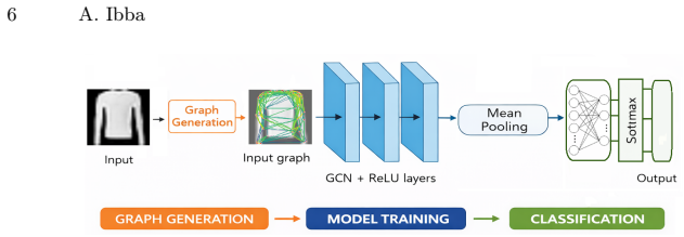


Reference graph
Works this paper leans on
-
[1]
In: Proceedings of the Sixth Workshop on Irregular Applications: Archi- tectures and Algorithms
Anastasiu, D.C., Karypis, G.: Fast parallel cosine k-nearest neighbor graph con- struction. In: Proceedings of the Sixth Workshop on Irregular Applications: Archi- tectures and Algorithms. p. 50–53. IA 16, IEEE Press (2016)
work page 2016
-
[2]
In: Rutkowski, L., Scherer, R., Korytkowski, M., Pedrycz, W., Tadeusiewicz, R., Zurada, J.M
Campos, W.S., Souza, L.G., Saito, P.T.M., Bugatti, P.H.: Contextual image clas- sification through fine-tuned graph neural networks. In: Rutkowski, L., Scherer, R., Korytkowski, M., Pedrycz, W., Tadeusiewicz, R., Zurada, J.M. (eds.) Artifi- cial Intelligence and Soft Computing. pp. 15–24. Springer International Publishing, Cham (2021)
work page 2021
-
[3]
Cao, P., Zhu, Z., Wang, Z., Zhu, Y., Niu, Q.: Applications of graph con- volutional networks in computer vision. Neural Comput. Appl.34(16), 13387–13405 (Aug 2022). https://doi.org/10.1007/s00521-022-07368-1, https://doi.org/10.1007/s00521-022-07368-1
-
[4]
Chen, Z.M., Wei, X.S., Wang, P., Guo, Y.: Multi-label image recognition with graph convolutional networks (2019), https://arxiv.org/abs/1904.03582 Visual graphs for image classification: does the structure affect performance? 13
work page internal anchor Pith review Pith/arXiv arXiv 2019
-
[5]
Dosovitskiy, A., Beyer, L., Kolesnikov, A., Weissenborn, D., Zhai, X., Unterthiner, T., Dehghani, M., Minderer, M., Heigold, G., Gelly, S., Uszkoreit, J., Houlsby, N.: An image is worth 16x16 words: Transformers for image recognition at scale (2021), https://arxiv.org/abs/2010.11929
work page internal anchor Pith review Pith/arXiv arXiv 2021
-
[6]
Edwards, M., Xie, X.: Graph based convolutional neural network (2016), https://arxiv.org/abs/1609.08965
work page internal anchor Pith review Pith/arXiv arXiv 2016
-
[7]
Han, K., Wang, Y., Guo, J., Tang, Y., Wu, E.: Vision gnn: An image is worth graph of nodes. In: NeurIPS (2022)
work page 2022
-
[8]
In: Schölkopf, B., Platt, J., Hoffman, T
Harel, J., Koch, C., Perona, P.: Graph-based visual saliency. In: Schölkopf, B., Platt, J., Hoffman, T. (eds.) Advances in Neural Information Processing Systems. vol. 19. MIT Press (2006)
work page 2006
-
[9]
He,K.,Zhang,X.,Ren,S.,Sun,J.:Deepresiduallearningforimagerecognition.In: Proceedings of the IEEE conference on computer vision and pattern recognition. pp. 770–778 (2016)
work page 2016
-
[10]
Jing, J., Gao, T., Zhang, W., Gao, Y., Sun, C.: Image feature in- formation extraction for interest point detection: A review (2022), https://arxiv.org/abs/2106.07929
work page internal anchor Pith review Pith/arXiv arXiv 2022
-
[11]
Kipf, T.N., Welling, M.: Semi-supervised classification with graph convolutional networks (2017), https://arxiv.org/abs/1609.02907
work page internal anchor Pith review Pith/arXiv arXiv 2017
-
[12]
Knyazev, B., Lin, X., Amer, M.R., Taylor, G.W.: Image classification with hierar- chical multigraph networks (2019), https://arxiv.org/abs/1907.09000
work page internal anchor Pith review Pith/arXiv arXiv 2019
-
[13]
Kosman, E., Oren, J., Castro, D.D.: Lsp : Acceleration and regularization of graph neural networks via locality sensitive pruning of graphs (2021), https://arxiv.org/abs/2111.05694
work page internal anchor Pith review Pith/arXiv arXiv 2021
-
[14]
In: Bengio, S., Wallach, H., Larochelle, H., Grauman, K., Cesa-Bianchi, N., Garnett, R
Li, Y., Gupta, A.: Beyond grids: Learning graph representations for visual recog- nition. In: Bengio, S., Wallach, H., Larochelle, H., Grauman, K., Cesa-Bianchi, N., Garnett, R. (eds.) Advances in Neural Information Processing Systems. vol. 31. Curran Associates, Inc. (2018)
work page 2018
-
[15]
In: 2021 International Conference on Information and Communication Technology Convergence (ICTC)
Linh, L.V., Youn, C.H.: Dynamic graph neural network for super-pixel im- age classification. In: 2021 International Conference on Information and Communication Technology Convergence (ICTC). pp. 1095–1099 (2021). https://doi.org/10.1109/ICTC52510.2021.9621101
-
[16]
Lowe, D.G.: Distinctive image features from scale-invariant keypoints. Int. J. Comput. Vision60(2), 91–110 (Nov 2004). https://doi.org/10.1023/B:VISI.0000029664.99615.94, https://doi.org/10.1023/B:VISI.0000029664.99615.94
-
[17]
Ma, X., Zhou, Y., Wang, H., Qin, C., Sun, B., Liu, C., Fu, Y.: Image as set of points (2023), https://arxiv.org/abs/2303.01494
work page internal anchor Pith review Pith/arXiv arXiv 2023
-
[18]
Nazir, U., Wang, H., Taj, M.: Survey of image based graph neural networks (2021), https://arxiv.org/abs/2106.06307
work page internal anchor Pith review Pith/arXiv arXiv 2021
-
[19]
Rodrigues, J., Carbonera, J.L.: Graph convolutional networks for im- age classification: Comparing approaches for building graphs from im- ages. In: International Conference on Enterprise Information Systems (2024), https://api.semanticscholar.org/CorpusID:269552841
work page 2024
-
[20]
Machine Learning and Knowledge Extrac- tion6, 2722–2737 (11 2024)
Shokouhinejad, H., Razavi-Far, R., Higgins, G., Ghorbani, A.: Node-centric prun- ing: A novel graph reduction approach. Machine Learning and Knowledge Extrac- tion6, 2722–2737 (11 2024). https://doi.org/10.3390/make6040130
-
[21]
In: European conference on computer vision
Wu, K., Zhang, J., Peng, H., Liu, M., Xiao, B., Fu, J., Yuan, L.: Tinyvit: Fast pretraining distillation for small vision transformers. In: European conference on computer vision. pp. 68–85. Springer (2022) 14 A. Ibba
work page 2022
-
[22]
Xiao, H., Rasul, K., Vollgraf, R.: Fashion-mnist: a novel image dataset for bench- marking machine learning algorithms (2017), https://arxiv.org/abs/1708.07747
work page internal anchor Pith review Pith/arXiv arXiv 2017
-
[23]
Computational Social Networks6(1), 11 (Nov 2019)
Zhang, S., Tong, H., Xu, J., Maciejewski, R.: Graph convolutional networks: a comprehensive review. Computational Social Networks6(1), 11 (Nov 2019). https://doi.org/10.1186/s40649-019-0069-y, https://doi.org/10.1186/s40649-019- 0069-y
-
[24]
Zhao, J., Yan, K., Zhao, Y., Guo, X., Huang, F., Li, J.: Transformer- based dual relation graph for multi-label image recognition (2021), https://arxiv.org/abs/2110.04722
work page internal anchor Pith review Pith/arXiv arXiv 2021
-
[25]
Artificial Intelligence Review 57(4), 99 (2024)
Zhao, X., Wang, L., Zhang, Y., Han, X., Deveci, M., Parmar, M.: A review of convolutional neural networks in computer vision. Artificial Intelligence Review 57(4), 99 (2024)
work page 2024
discussion (0)
Sign in with ORCID, Apple, or X to comment. Anyone can read and Pith papers without signing in.