REVIEW 3 major objections 5 minor 24 references
A single optimization with an explainability-aware L0 penalty both explains misclassifications and measures how far a classifier can be pushed under human-readable changes.
Reviewed by Pith at T0; open to challenge. T0 means a machine referee read the full paper against a public rubric. the ladder, T0–T4 →
An explainability-aware L0 penalty yields coherent counterfactual edits, and the same geometry defines a Tolerance-Region Confusion Matrix that quantifies class-to-class fragility under interpretable perturbations.
T0 review reviewed 2026-07-11 challenge →
load-bearing objection Clean methods paper that couples domain-structured sparsity into counterfactuals and ships a usable robustness matrix; the interpretability claim is only as strong as the hand-designed W. the 3 major comments →
Optimized Instance Alteration for Explaining and Assessing Robustness of Classifiers
The pith
A machine-rendered reading of the paper's core claim, the machinery that carries it, and where it could break.
The reading
Core claim
The authors establish that a composite objective combining a classification hinge, a proximity term, and a novel explainability-aware L0 (XA-L0) penalty produces minimal, structured counterfactual corrections that both diagnose misclassification and, when used to define tolerance regions, yield a Tolerance-Region Confusion Matrix that quantifies class-to-class transition probabilities under interpretable perturbations, revealing robustness differences invisible to standard accuracy or adversarial metrics.
What carries the argument
Explainability-aware L0 (XA-L0) penalty: a differentiable pairwise product of soft activations weighted by an incoherence matrix W that couples correlated features, feature communities, spatially near pixels, or edge pixels; the same penalty geometry defines the tolerance regions whose reachable-class counts form the TOR-Confusion Matrix.
Load-bearing premise
The hand-chosen weights that couple features or pixels (correlations, communities, distances, edge maps) really do capture the structure humans find meaningful, so that minimizing the penalty actually produces interpretable edits.
What would settle it
On a fixed set of misclassified tabular or image instances, measure whether human raters consistently judge XA-L0 edits more coherent and actionable than matched L0 or L2 baselines, and whether TOR-CM off-diagonal rates predict actual label flips under the same structured budgets; failure of either comparison would undermine the central claim.
If this is right
- Counterfactual corrections become compact groups of related features or edge-aligned pixel clusters rather than scattered isolated changes.
- A single optimization run can both flip a misclassified instance to the true label and supply a binary mask explaining which coordinates caused the original error.
- TOR-CM supplies per-class reachability probabilities under a shared interpretable budget, allowing models of similar accuracy to be ranked by how quickly off-diagonal transitions appear as the budget grows.
- High-accuracy models such as CNNs can be shown to be more fragile under structured edits than lower-accuracy but more stable classical models such as random forests.
- The same framework can flag borderline decisions that hinge on only a few coherent factors, supporting debugging or policy review.
Where Pith is reading between the lines
- If the W matrix can be learned from user feedback rather than fixed a priori, the same optimizer could adapt explanations to domain experts without redesigning the penalty.
- TOR-CM reachability counts could serve as a training regularizer, penalizing models whose decision regions are too easily escaped under structured budgets.
- The method naturally extends to mixed categorical-numeric data once a suitable discrete-to-continuous relaxation of XA-L0 is defined, a direction left open by the authors.
- Comparing TOR-CM vulnerability across model families on the same data may give a practical alternative to pure adversarial robustness certificates when the threat model is human-scale edits rather than noise.
Editorial analysis
A structured set of objections, weighed in public.
Referee Report
Summary. The paper proposes a unified optimization framework for generating interpretable counterfactual corrections of black-box classifiers and for assessing their robustness under structured perturbations. The composite objective (Eqs. 1–5) combines a classification hinge, an L2 proximity term, and a novel explainability-aware L0 (XA-L0) penalty (Eq. 6) whose pairwise weights W_ij encode feature affinity (Pearson correlation or spectral communities for tabular data; spatial distance or HED edge maps for images). After gradient optimization and post-hoc zero-clipping, the resulting sparse edits are used both as explanations of misclassifications and to define tolerance regions. Robustness is summarized by the Tolerance-Region Confusion Matrix (TOR-CM, Eqs. 8–11) and the aggregate metrics γ_a, γ_v. Experiments on seven tabular datasets, MNIST, and Flowers-102 compare XA-L0 against L0/L2 baselines, a Dandl-inspired scalarization, CEM/CEMAE, and SEDC, reporting lower structural incoherence φ(S) (Eq. 7) and sparsity n, plus TOR-CM differences across classifiers that standard confusion matrices miss.
Significance. If the claims hold, the work supplies a single, differentiable objective that simultaneously produces structured counterfactuals and a class-transition view of robustness under human-aligned rather than adversarial perturbations. The explicit construction of XA-L0, the structural-incoherence score, and TOR-CM are concrete, reusable contributions; the experimental design (fixed budgets, shared thresholding, multiple affinity constructions) is careful enough to make the empirical patterns informative. The main limitation is that interpretability is measured only by fidelity to the hand-designed W matrices, so the practical value of the framework for real decision-makers remains to be established by human or domain-expert validation.
major comments (3)
- The central claim that XA-L0 yields more interpretable corrections rests on lower φ(S) (Eq. 7) and sparsity n (Table II, Figs. 1–4). Both quantities are defined from the same pairwise weights W_ij that appear inside the XA-L0 regularizer itself (§III-B). Consequently the reported gains largely show that the optimizer respects the structure it was told to respect; they do not independently establish that those structures match human notions of semantic meaningfulness. No human judgment study, alternative affinity ablation, or domain-expert annotation is provided. Without such external validation the interpretability claim (and the assertion that TOR-CM measures robustness under “interpretable” perturbations) remains only partially grounded.
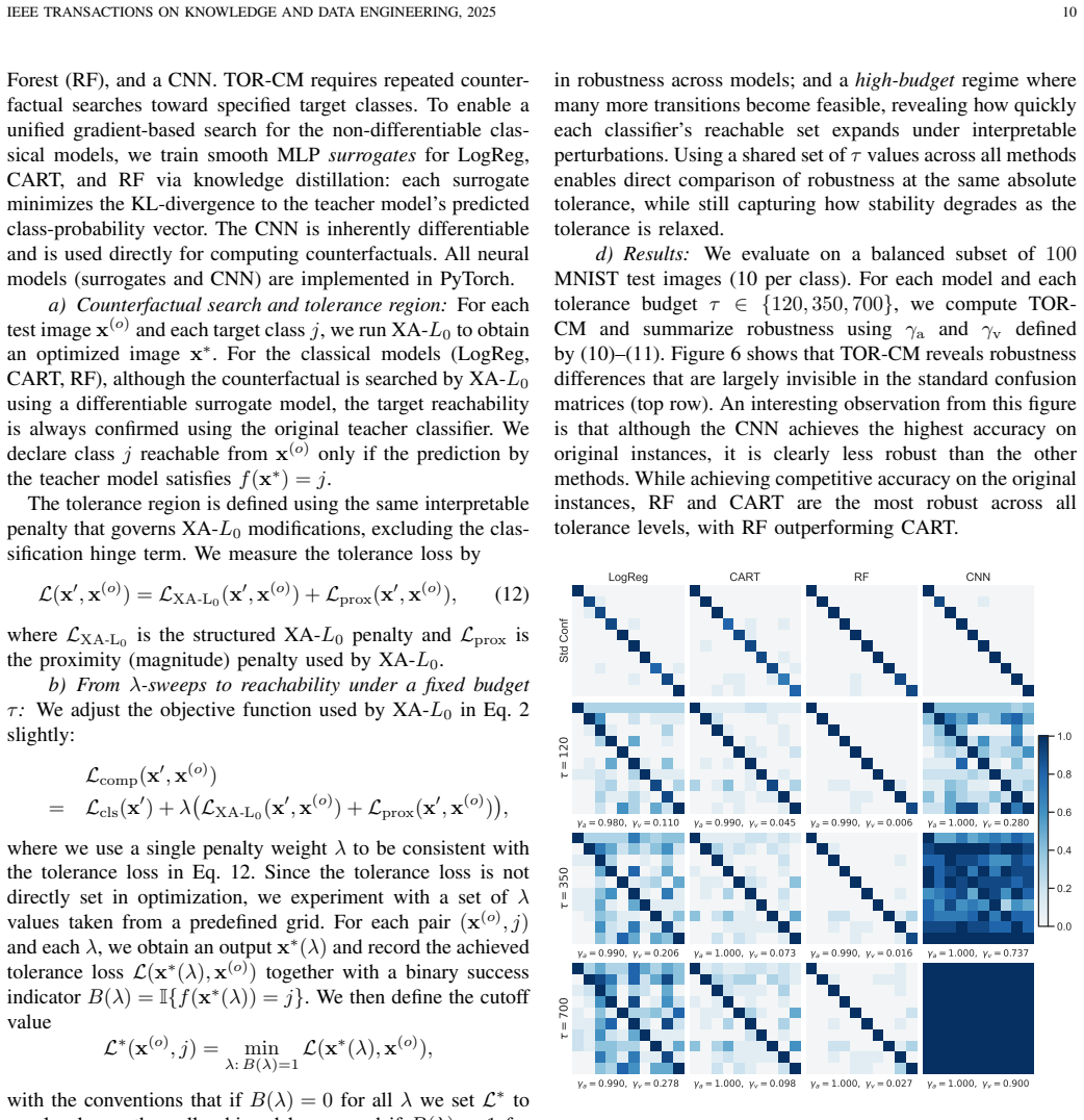
- TOR-CM for non-differentiable models (LogReg, CART, RF) is obtained by searching with distilled MLP surrogates while confirming labels with the teacher (§IV-D). The manuscript does not report surrogate fidelity (e.g., agreement rate or KL divergence on the test set) nor quantify how often a surrogate-found x* fails the teacher check. Because reachability indicators and the resulting γ_v values depend on this pipeline, the robustness ranking (CNN least robust, RF most robust) could be an artifact of surrogate approximation error rather than a property of the original classifiers.
- Tolerance budgets τ ∈ {120, 350, 700} for MNIST (§IV-D) and the single shared τ used for the toy example are presented without a principled selection procedure or sensitivity analysis. Because γ_v and the off-diagonal mass of TOR-CM grow rapidly with τ, the qualitative conclusion that CNN is markedly less robust than RF/CART is sensitive to these particular cut-offs. A brief calibration (e.g., quantiles of achieved L under successful flips, or a continuous au-sweep) is needed to show that the ranking is stable.
minor comments (5)
- Notation for the soft activation σ and the edge-aware weights (α_edge, W_ed_i) is introduced without a single consolidated hyper-parameter table; readers must hunt through §III-B and the experimental paragraphs for ξ, ζ, au, κ, ε, au_clip.
- Figure 1 bins instances by L2 and plots mean ± std of φ and n; the number of instances per bin is never stated, making it hard to judge whether the shaded bands are reliable.
- The optional classification margin θ appears in the text after Eq. (3) but is never used or ablated in the reported experiments; either drop it or show its effect.
- References [8] and [10] appear to be the same survey; consolidate to avoid duplication.
- In §IV-A the community count K_c = max{2, min(d-1, round(√d))} is reasonable but never justified or compared with other choices of K_c.
Circularity Check
φ(S) and edge-distance metrics are built from the same hand-designed W (or edge map) that defines the XA-L0 regularizer, so reported coherence gains are partly by construction of the objective.
specific steps
-
self definitional
[§III-B Eq. (6) and §III-D Eq. (7); Table II / Fig. 1]
"L_XA-L0(x,x(o)) = ∑_{(i,j)∈I} W_{i,j} σ(|x_i−x_i^{(o)}|)σ(|x_j−x_j^{(o)}|) φ(S)=1/(d|S|) ∑_{i∈S} ∑_{j∈S} exp(ψ W_{i,j})"
W is the same matrix that appears inside the objective being minimized and inside the post-hoc coherence score. Selecting a support that activates low-W pairs necessarily yields a small φ(S). The large φ gaps versus L2+Lcls baselines in Table II and Fig. 1 are therefore largely forced by the choice of regularizer rather than an independent demonstration of semantic interpretability.
-
self definitional
[§III-B (edge-focused) and Fig. 4]
"W_ed_i = ε+(1−ε)(1−α̃_edge(i)), L_ed_XA-L0 = ∑ W_ed_i σ(|x_i−x_i^{(o)}|) [Fig. 4] mean distance of changed pixels to the nearest detected edge"
The edge-aware penalty explicitly down-weights non-edge pixels; the reported “mean distance to edges” metric therefore decreases by construction whenever the optimizer succeeds. The claim that XA-L0 produces more “visually coherent / edge-aligned” corrections is measured by the same structure the method was told to respect.
full rationale
The paper is a methods contribution (optimization + new matrix), not a first-principles derivation of a physical law, so full circularity is not expected. The optimization itself is self-contained: L_cls forces a label flip, L_prox and the soft-L0 surrogate are standard, and success is checked by the black-box classifier. TOR-CM reachability counts are likewise empirical under a fixed budget. The only circular step is the evaluation of “structural coherence / interpretability”: both the regularizer L_XA-L0 (Eq. 6) and the reported metric φ(S) (Eq. 7) are defined from the identical pairwise matrix W (Pearson / communities for tables; spatial Gaussian or HED edge map for images). Minimizing the regularizer therefore tends to produce supports S whose φ is low by design; the same holds for the mean edge-distance reported on Flowers-102. This is a mild self-definitional loop that inflates the quantitative claim of superior interpretability, but it does not force the label-flip success, the sparsity numbers n, the visual examples, or the TOR-CM robustness rankings. No self-citation chain, uniqueness theorem, or fitted-parameter-as-prediction is present. Score 3 reflects one clear but non-central circularity of metric construction.
Axiom & Free-Parameter Ledger
free parameters (8)
- λ1, λ2 (or single λ) regularization weights
- ξ soft-activation steepness
- ζ spatial Gaussian bandwidth
- edge-aware hyperparameters (α_min, τ, κ, ε)
- post-hoc zero-clip threshold t
- community penalties ω_in, ω_out and K_c
- tolerance budgets τ for TOR-CM
- classification margin θ (optional)
axioms (5)
- domain assumption A differentiable soft product of pairwise activations is a valid surrogate for structured L0 sparsity suitable for gradient-based counterfactual search.
- ad hoc to paper Feature affinity from Pearson correlation or spectral communities (tabular) and spatial/edge proximity (images) is the right geometry for human-interpretable edits.
- ad hoc to paper Tolerance regions defined by L_XA-L0 + L_prox (not adversarial ℓ_p balls) are the appropriate notion of robustness for the paper’s claims.
- domain assumption For non-differentiable teachers, reachability confirmed on the teacher after search on a distilled MLP surrogate is a valid robustness measurement.
- standard math Standard optimization and clustering tools (ADAM, spectral clustering, HED edges) behave as expected for the reported experiments.
invented entities (3)
-
Explainability-Aware L0 (XA-L0) penalty
no independent evidence
-
Tolerance-Region Confusion Matrix (TOR-CM)
no independent evidence
-
Structural incoherence score φ(S)
no independent evidence
Cite this review
Pith. "Pith review of Optimized Instance Alteration for Explaining and Assessing Robustness of Classifiers." pith.science (2026). https://pith.science/paper/PJP5W7QQ
@misc{pith2026260706637,
  author       = {Pith},
  title        = {Pith review of: Optimized Instance Alteration for Explaining and Assessing Robustness of Classifiers},
  year         = {2026},
  howpublished = {\url{https://pith.science/paper/PJP5W7QQ}},
  note         = {Machine review of arXiv:2607.06637}
}
abstract
In this work, we propose a unified approach for diagnosing misclassification and assessing the robustness of black-box classifiers. Central to our method is an optimization framework that modifies an instance so that the classifier predicts a specified target label, while ensuring that the modification remains easily explainable. The objective function contains two components: an explainability-aware $L_0$ (XA-$L_0$) penalty that promotes sparse and interpretable modifications, and a classifier loss objective that steers the perturbed instance toward the desired output. This integrated optimization formulation is used both to identify the underlying causes of misclassification and to evaluate robustness by determining how an instance can change within a tolerance region before being reassigned to another class. To quantify robustness, we introduce the Tolerance Region Confusion Matrix (TOR-Confusion Matrix), which measures a classifier's susceptibility by modeling the class-to-class transition probabilities induced by tolerance-bounded perturbations. We validate the proposed method on both image and tabular datasets, demonstrating its ability to jointly deliver interpretability and robustness assessment.
Figures


Reference graph
Works this paper leans on
-
[1]
Counterfactual explanations without opening the black box: Automated decisions and the gdpr,
S. Wachter, B. Mittelstadt, and C. Russell, “Counterfactual explanations without opening the black box: Automated decisions and the gdpr,” Harvard Journal of Law & Technology, vol. 31, no. 2, pp. 841–887, 2017
work page 2017
-
[2]
Desiderata for interpretable explanations: Quantifying interpretability of explanations,
A. Dhurandhar, P.-Y . Chen, R. Luss, C.-C. Tu, P. Ting, K. Shanmugam, and P. Das, “Desiderata for interpretable explanations: Quantifying interpretability of explanations,” inProceedings of the 2018 IEEE International Conference on Data Mining (ICDM). IEEE, 2018, pp. 1103–1108
work page 2018
-
[3]
Multi-objective counter- factual explanations,
S. Dandl, C. Molnar, M. Binder, and B. Bischl, “Multi-objective counter- factual explanations,”Machine Learning, vol. 110, no. 3, pp. 495–507, 2021
work page 2021
-
[4]
Inverse Classification for Comparison-based Interpretability in Machine Learning
T. Laugel, M.-J. Lesot, C. Marsala, X. Renard, and M. Detyniecki, “Inverse classification for comparison-based interpretability in machine learning,”arXiv preprint arXiv:1712.08443, 2017
work page internal anchor Pith review Pith/arXiv arXiv 2017
-
[5]
Explaining and harnessing adversarial examples,
I. J. Goodfellow, J. Shlens, and C. Szegedy, “Explaining and harnessing adversarial examples,” inInternational Conference on Learning Repre- sentations (ICLR), 2015
work page 2015
-
[6]
Towards deep learning models resistant to adversarial attacks,
A. Madry, A. Makelov, L. Schmidt, D. Tsipras, and A. Vladu, “Towards deep learning models resistant to adversarial attacks,” inInternational Conference on Learning Representations (ICLR), 2018
work page 2018
-
[7]
Certified adversarial robustness via randomized smoothing,
J. Cohen, E. Rosenfeld, and J. Z. Kolter, “Certified adversarial robustness via randomized smoothing,” inInternational Conference on Machine Learning (ICML). PMLR, 2019, pp. 1310–1320
work page 2019
-
[8]
Counterfactual explanations and algorithmic recourses for machine learning: A review,
S. Verma, V . Boonsanong, M. Hoang, K. Hines, J. Dickerson, and C. Shah, “Counterfactual explanations and algorithmic recourses for machine learning: A review,”ACM Computing Surveys, vol. 56, no. 12, pp. 1–42, 2024
work page 2024
-
[9]
Algorithmic recourse: from counterfactual explanations to interventions,
A.-H. Karimi, B. Sch ¨olkopf, and I. Valera, “Algorithmic recourse: from counterfactual explanations to interventions,” inProceedings of the 2021 ACM conference on fairness, accountability, and transparency, 2021, pp. 353–362
work page 2021
-
[10]
Counterfactual explanations and algorithmic recourses for machine learning: A review,
S. Verma, V . Boonsanong, M. Hoang, K. Hines, J. Dickerson, and C. Shah, “Counterfactual explanations and algorithmic recourses for machine learning: A review,”ACM Comput. Surv., vol. 56, no. 12, Oct
-
[11]
Available: https://doi.org/10.1145/3677119
[Online]. Available: https://doi.org/10.1145/3677119
-
[12]
Explaining machine learning classifiers through diverse counterfactual explanations,
R. K. Mothilal, A. Sharma, and C. Tan, “Explaining machine learning classifiers through diverse counterfactual explanations,” inProceedings of the 2020 conference on fairness, accountability, and transparency, 2020, pp. 607–617
work page 2020
-
[13]
Getting a CLUE: A Method for Explaining Uncertainty Estimates
J. Antor ´an, U. Bhatt, T. Adel, A. Weller, and J. M. Hern ´andez-Lobato, “Getting a clue: A method for explaining uncertainty estimates,”arXiv preprint arXiv:2006.06848, 2020
work page internal anchor Pith review Pith/arXiv arXiv 2006
-
[14]
S. Joshi, O. Koyejo, W. Vijitbenjaronk, B. Kim, and J. Ghosh, “Towards realistic individual recourse and actionable explanations in black-box decision making systems,”arXiv preprint arXiv:1907.09615, 2019
work page internal anchor Pith review Pith/arXiv arXiv 1907
-
[15]
Interpretable counterfactual explana- tions guided by prototypes,
A. Van Looveren and J. Klaise, “Interpretable counterfactual explana- tions guided by prototypes,” inJoint European Conference on Machine Learning and Knowledge Discovery in Databases. Springer, 2021, pp. 650–665
work page 2021
-
[16]
Model selection and estimation in regression with grouped variables,
M. Yuan and Y . Lin, “Model selection and estimation in regression with grouped variables,”Journal of the Royal Statistical Society: Series B (Statistical Methodology), vol. 68, no. 1, pp. 49–67, 2006
work page 2006
-
[17]
Sparsity and smoothness via the fused lasso,
R. Tibshirani, M. Saunders, S. Rosset, J. Zhu, and K. Knight, “Sparsity and smoothness via the fused lasso,”Journal of the Royal Statistical Society: Series B (Statistical Methodology), vol. 67, no. 1, pp. 91–108, 2005
work page 2005
-
[18]
S. Kim, K.-A. Sohn, and E. P. Xing, “Multivariate regression with grouped variables: Modeling and estimation via sparse graphical mod- els,”Journal of Machine Learning Research, vol. 10, pp. 513–546, 2009
work page 2009
-
[19]
A tutorial on spectral clustering,
U. V on Luxburg, “A tutorial on spectral clustering,”Statistics and computing, vol. 17, no. 4, pp. 395–416, 2007
work page 2007
-
[20]
Modularity and community structure in networks,
M. E. J. Newman, “Modularity and community structure in networks,” Proceedings of the National Academy of Sciences, vol. 103, no. 23, pp. 8577–8582, 2006
work page 2006
-
[21]
Holistically-nested edge detection,
S. Xie and Z. Tu, “Holistically-nested edge detection,” inProceedings of the IEEE international conference on computer vision, 2015, pp. 1395– 1403
work page 2015
-
[22]
Explanations based on the missing: Towards contrastive explanations with pertinent negatives,
A. Dhurandhar, P.-Y . Chen, R. Luss, C.-C. Tu, P. Ting, K. Shanmugam, and P. Das, “Explanations based on the missing: Towards contrastive explanations with pertinent negatives,”Advances in neural information processing systems, vol. 31, 2018
work page 2018
-
[23]
Explainable image classification with evidence counter- factual,
T. Vermeire, D. Brughmans, S. Goethals, R. M. B. De Oliveira, and D. Martens, “Explainable image classification with evidence counter- factual,”Pattern Analysis and Applications, vol. 25, no. 2, pp. 315–335, 2022. Evgenii Kuriabovis a Ph.D. candidate in the De- partment of Statistics at The Pennsylvania State Uni- versity. His research interests include i...
work page 2022
-
[24]
He was General Chair for the 2001 IEEE Workshop on Neural Networks for Signal Processing
He was an Associate Editor for IEEE Transactions on Signal Processing from 2004-2007. He was General Chair for the 2001 IEEE Workshop on Neural Networks for Signal Processing. Jia Li(Fellow, IEEE) is a Professor of Statistics and (by courtesy) Computer Science and Engineering at The Pennsylvania State University. Her research interests include machine lea...
work page 2004
This paper was first reviewed by grok-4.5 on July 11, 2026.
discussion (0)
Sign in with ORCID, Apple, or X to comment. Anyone can read and Pith papers without signing in.