REVIEW 1 major objections 7 minor 32 references
Reviewed by Pith at T0; open to challenge.
T0 means a machine referee read the full paper against a public rubric. The mark states how deep the mechanical check went, never who wrote it. the ladder, T0–T4 →
load-bearing objection Real problem, reasonable architecture, but the two headline accuracy metrics are artifacts of data distribution and degenerate prediction behavior — not evidence of genuine forecasting capability. the 1 major comments →
Agent Delivery Engineering Predictive Reliability Framework
The pith
A machine-rendered reading of the paper's core claim, the machinery that carries it, and where it could break.
Core claim
The central object is the Trust Margin (TM) score — a single scalar (0–100) computed from 20 behavioral metadata signals (process liveness, tool-call patterns, state consistency, verification pass rates, entropy rate) aggregated across five weighted layers (Survival 0.30, Order 0.30, Credibility 0.25, Guardianship 0.10, Posture 0.05). The core mechanism is that agent system degradation follows a progressive, cumulative disorder pattern rather than discrete failure events, and that this disorder can be tracked through purely mathematical operations on behavioral metadata — no LLM inference, no semantic parsing of outputs, no access to dialogue content. The prediction engine (ETA 3.1.0) runs a
What carries the argument
TM score (0–100) from 20 signals across 5 weighted layers; ETA 3.1.0 three-stage prediction (Kalman → Survival Analysis → Exponential Smoothing); MCP Server sidecar deployment; zero-LLM, zero-semantic-intrusion computation (<2.5 ms per scoring, ~150 KB memory); four-tier decision boundaries (Safe >85, Watch 70–85, Alert 50–70, Circuit-Break <50) with hysteresis; adaptive α calibration achieving 20× MAE improvement (13.73 → 0.66); AOC remediation module for closed-loop monitoring→diagnosis→repair
Load-bearing premise
The five-layer weight allocation (L1=0.30, L2=0.30, L3=0.25, L4=0.10, L5=0.05) and the 20-signal aggregation formula are calibrated on the same production deployment used for validation, based on 'engineering judgment' rather than independent data. With only 2 severe degradation events observed in 15 days, the weights have minimal empirical grounding. If these weights do not generalize to other agent architectures or deployment contexts, the TM score's diagnostic value andETA
What would settle it
Deploy TM 3.1.0 on an independent agent platform (different LLM provider, different task domain, different framework) without recalibrating the five-layer weights. If the TM score does not couple with ground-truth degradation states — or if the Exponential method's direction accuracy drops substantially below 76.8% — the framework's generalization claim fails. Alternatively, if CADVP_PASS (the identified 'canary' signal) does not show early sensitivity to degradation on the new platform, the factor ranking may be deployment-specific rather than universal.
If this is right
- If the TM framework generalizes, production agent deployments could shift from reactive incident response to predictive maintenance — issuing warnings hours before visible failure, analogous to how aerospace and industrial reliability engineering use safety margins to anticipate breakdowns.
- The finding that Exponential smoothing outperforms Kalman filtering for agent health prediction suggests that agent degradation dynamics differ structurally from the stationary-state assumptions underlying Kalman models — degradation is predominantly downward-trending rather than mean-reverting, which has implications for any forecasting approach applied to agent reliability.
- The 'false prosperity' phenomenon, if confirmed beyond this deployment, implies that current industry-standard observability tools (APM systems, LLM tracing platforms) are systematically blind to the most dangerous degradation mode in agent systems — a gap that cannot be closed by adding more metric dimensions to existing tools.
- The CADVP_PASS signal (cross-agent verification pass rate) identified as the most sensitive degradation 'canary' could become a standard early-warning metric adopted independently of the full TM framework, giving operations teams a single high-signal indicator to monitor.
Where Pith is reading between the lines
- The framework's weight calibration rests on only 2 severe degradation events in 15 days, meaning the five-layer weight allocation (0.30/0.30/0.25/0.10/0.05) is essentially an engineering prior, not an empirically derived optimum. Whether these weights transfer to agent systems with different architectures, model providers, or task profiles is untested. A natural extension would be to deploy TM acr
- The observation that 73.9% of telemetry sequences have optimal α=0 (pure mean prediction) suggests that during normal operation, most agent signals carry no degradation information — they are pure noise. This raises the question of whether a simpler anomaly-detection approach (statistical process control on a few high-sensitivity signals like CADVP_PASS) could achieve comparable early-warning perf
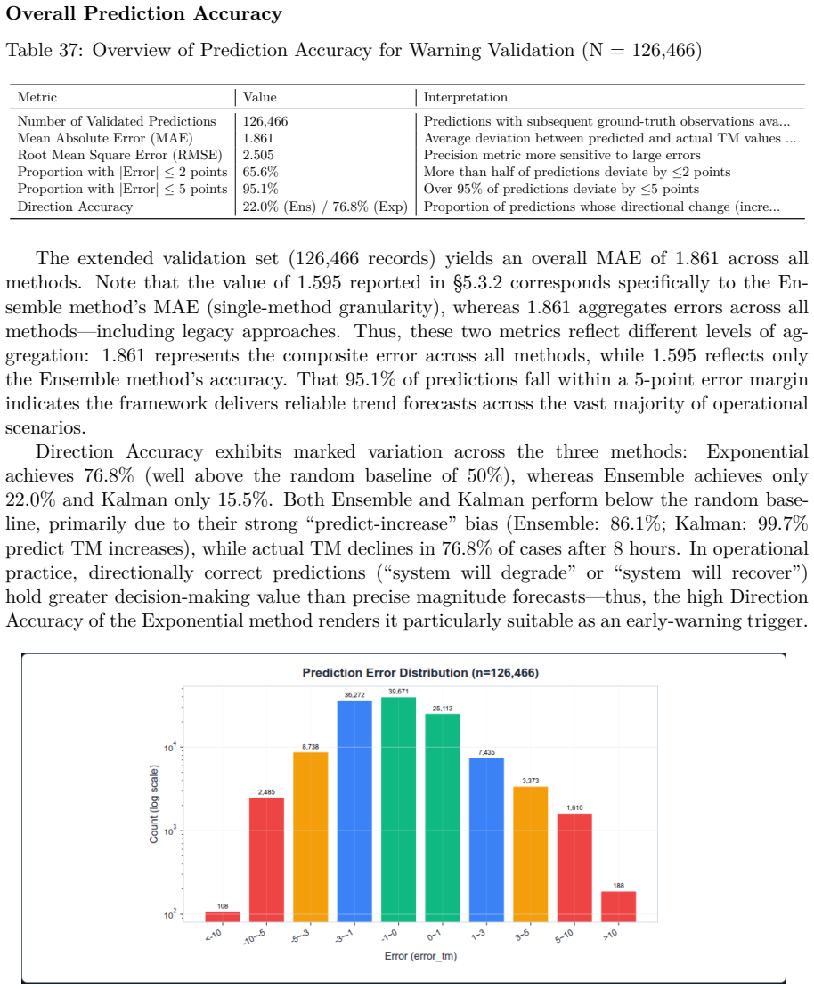
- The Exponential method's 100% 'predict decrease' strategy achieving 76.8% direction accuracy is partly a consequence of the dataset's base rate: TM declines in 76.8% of 8-hour windows. This means the method's direction accuracy may be an artifact of always predicting decline rather than genuinely discriminating degradation direction. A more informative test would be direction accuracy on balanced
- The paper's positioning as 'among the earliest' predictive reliability frameworks for LLM agents suggests the field is at a stage where establishing the problem formulation and demonstrating feasibility on a single deployment is the contribution — not yet proving generality. The framework's value proposition depends on whether the TM score's coupling with ground-truth states (observed upon ADE plu
Editorial analysis
A structured set of objections, weighed in public.
Referee Report
Summary. The paper proposes ADE-PRF, a framework for quantifying and predicting the reliability of LLM-based multi-agent systems. It introduces a Trust Margin (TM) score computed from 20 behavioral-metadata signals aggregated across five architectural layers, and an ETA prediction engine that forecasts TM values over an 8-hour horizon using Kalman filtering, survival analysis, and exponential smoothing. The framework is validated on 15 days of production data from six agent profiles on the Hermes platform (154,906 predictions), supplemented by five controlled sandbox degradation experiments. The paper is the fourth in a series building a theory-to-engineering pipeline for agent reliability. The system-level monitoring concept and the zero-semantic-intrusion design are interesting engineering contributions. However, the central accuracy claims rest on metrics that are substantially inflated by the data's distributional properties and by a degenerate prediction strategy, which the paper does not adequately disclose or address.
Significance. The paper tackles a genuine and timely problem: runtime reliability monitoring for LLM agent systems that goes beyond infrastructure-level observability. The zero-LLM, zero-semantic-intrusion design (§3.5) is a principled engineering choice that avoids the circularity of using an LLM to evaluate LLM reliability, and the reported computational overhead (<2.5 ms per scoring cycle, ~150 KB memory) is commendably low. The five-layer decomposition with interpretable backtracking is a reasonable architectural decision. The sandbox degradation experiments (§5.5, Table 36) show prediction errors of ≤0.3 points across five injected patterns, which—if they hold up under independent replication—would be a meaningful result. The paper also provides falsifiable predictions (specific MAE and Direction Accuracy targets) and is transparent about several limitations, including the backtesting caveat in §5.6. However, the significance is substantially undermined by the evaluation issues detailed below.
major comments (1)
- §5.6.3, Table 40: The Exponential method's headline Direction Accuracy of 76.8% is achieved by predicting 'decrease' in 100.0% of cases, while TM actually decreases in 76.8% of cases. This is a degenerate majority-class predictor that provides zero discriminative signal—it cannot distinguish cases where TM will decrease from cases where it will increase or remain stable. The paper acknowledges this pattern but frames it as a feature ('particularly suitable as an early-warning trigger,' §5.6.3). A constant predictor that always outputs the majority class is not evidence of predictive capability. This is load-bearing because Direction Accuracy is one of only two headline accuracy metrics (alongside MAE=1.228), and the paper's claim of 'forward-looking warning capability' depends on it. The paper must either (a) report Direction Accuracy relative to the base rate (i.e., show that the Ex-ESM
minor comments (7)
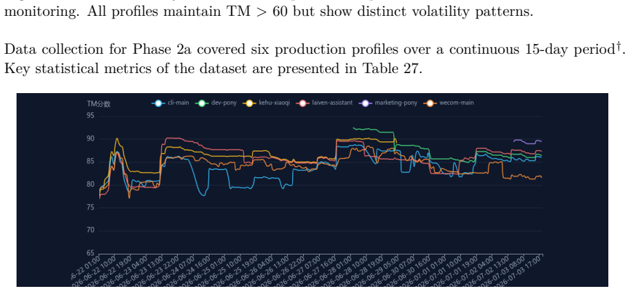
- The abstract states '380,227 predictions and 280,579 validations' but §5.3 (Table 27) reports 154,906 predictions with 126,466 validated. The discrepancy should be reconciled or the abstract corrected.
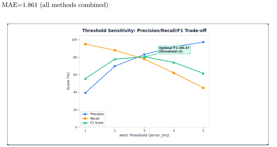
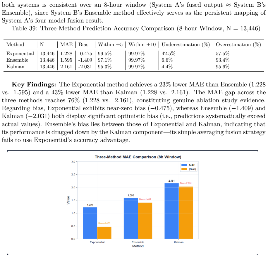
- Table 1 reports '8h Lookahead MAE 1.861 (all methods combined)' but later sections report 1.595 (Ensemble) and 1.228 (Exponential). The relationship between these numbers should be stated explicitly in the table caption or the main text to avoid confusion.
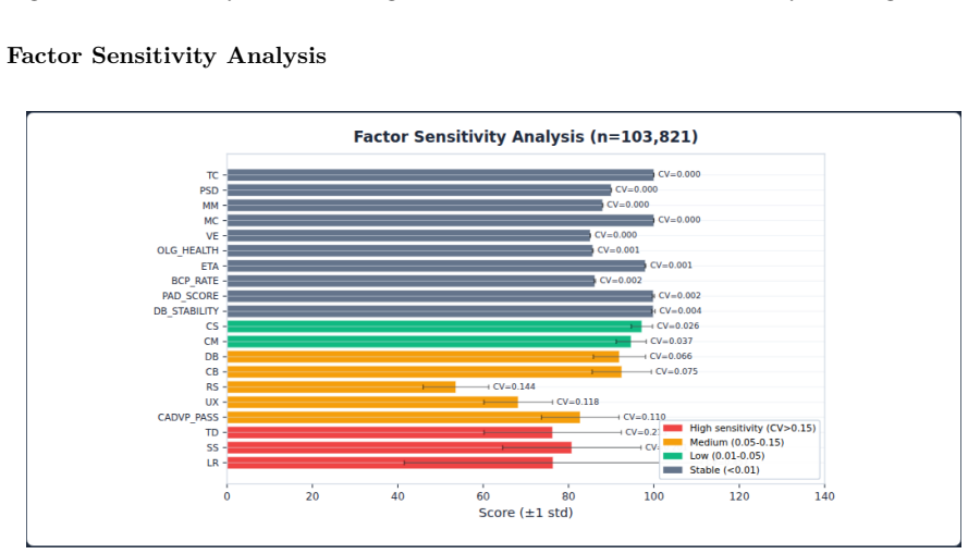
- §3.3.2 references 'PAD' in the text description of L2 Order Layer but the signal is listed as 'PAD_SCORE' in Table 12 (L3 Credibility Layer). This appears to be a cross-referencing error.
- The paper mentions 'seven sandbox-controlled experiments' in the abstract but §5.5 (Table 36) describes five degradation patterns. The text in §5.2 mentions expansion to seven sandboxes but this is not clearly tabulated. Either the abstract should say five or the additional two experiments should be documented.
- §5.3, Table 30: The MAE values per profile (cli-main=3.033, kehu-xiaoqi=0.822) are described with qualitative labels ('Best,' 'Excellent,' 'Good,' 'Acceptable') that are inconsistent—cli-main has the highest MAE but is labeled 'Best,' while kehu-xiaoqi has the lowest MAE but is labeled 'Good.' The labels should be corrected or clarified.
- The paper is the fourth in a series referencing three prior works [1, 2, 3] by the same author. While the relationship is explained in §1, the prior works appear to be arXiv preprints from the same period (June 2026). The paper should clarify whether these have undergone peer review.
- Figure numbering and references are inconsistent in places (e.g., §6 appears multiple times in the organization section). The section numbering should be corrected.
Simulated Author's Rebuttal
We thank the referee for a careful and substantive reading. The referee's central criticism — that the Exponential method's Direction Accuracy of 76.8% is an artifact of a degenerate majority-class predictor — is correct. We accept this point and will revise the manuscript accordingly. We also clarify which claims survive this criticism and which do not.
read point-by-point responses
-
Referee: §5.6.3, Table 40: The Exponential method's headline Direction Accuracy of 76.8% is achieved by predicting 'decrease' in 100.0% of cases, while TM actually decreases in 76.8% of cases. This is a degenerate majority-class predictor that provides zero discriminative signal. The paper frames this as a feature ('particularly suitable as an early-warning trigger'). Direction Accuracy is one of only two headline accuracy metrics (alongside MAE=1.228), and the claim of 'forward-looking warning capability' depends on it. The paper must either (a) report Direction Accuracy relative to the base rate, or otherwise address the degeneracy.
Authors: The referee is correct. We acknowledge this without reservation. The Exponential method predicts 'decrease' in 100.0% of cases, and the actual base rate of decrease is 76.8%. Therefore the reported Direction Accuracy of 76.8% carries zero discriminative information — it is exactly the majority-class base rate. A constant predictor that always outputs the majority class is not evidence of predictive capability, and our framing of this as 'particularly suitable as an early-warning trigger' was misleading. We will revise the manuscript as follows: (1) We will explicitly state that the Exponential method's Direction Accuracy equals the base rate and therefore provides no discriminative signal beyond majority-class prediction. (2) We will remove or heavily qualify the claim that Direction Accuracy demonstrates 'forward-looking warning capability' for the Exponential method. (3) We will report Direction Accuracy relative to the base rate (i.e., excess accuracy over the majority-class baseline) for all three methods, making clear that Exponential's excess accuracy is 0.0 percentage points. (4) We will remove Direction Accuracy from the abstract as a headline metric and retain MAE as the primary accuracy claim. (5) The stratified analysis in Table 41 does not rescue the claim: if the method always predicts 'decrease,' higher accuracy on larger-magnitude strata merely reflects that larger changes are more likely to be decreases — not that the method discriminates. We will state this limitation explicitly. What does survive: The MAE=1.228 for the Exponential method measures absolute error magnitude and is not affected by the direction-prediction degeneracy. The sandbox controlled-degradation results (Table 36, prediction errors ≤0.3 points across five injected patterns) are also, revision: no
Circularity Check
Two circular steps: (1) the '20× MAE improvement' from adaptive α calibration is measured on the same data used to optimize α, and (2) the Exponential method's headline Direction Accuracy of 76.8% is identical to the base rate of actual decreases, achieved by predicting 'decrease' 100% of the time.
specific steps
-
fitted input called prediction
[§4.4, Table 21-22, and §5.3.3 Table 31]
"Table 21: Statistical Distribution of Smoothing Parameter α... Proportion of α=0: 73.9%... Note: The α statistics in Tables 20–21 reflect per-sequence optimal smoothing parameters determined during online learning within the ETA engine... Table 22: Prediction Accuracy Before and After Adaptive Calibration: MAE (Mean) 13.73 → 0.66, 20.8× improvement... primarily driven by online optimization of the α parameter. The adaptive mechanism independently optimizes α for each sequence, resolving this trade-off."
The α parameter is optimized per-sequence on the same production data that is then used to evaluate prediction accuracy. The paper explicitly states α is 'per-sequence optimal smoothing parameters determined during online learning' and then reports the '20× MAE improvement' (13.73→0.66) as evidence of the framework's adaptive capability. Since α is fit to each sequence and then evaluated on that same sequence, the MAE improvement measures in-sample fit quality, not generalization. The paper itself flags this as backtesting with 'risk of future data leakage' (§5.6), but the headline '20× improvement' is still presented as a core result.
-
self definitional
[§5.6.3, Table 40]
"Table 40: Direction Accuracy Comparison Across Three Prediction Methods — Exponential: Direction Accuracy 76.8%, % Predicted Increase 0.0%, % Predicted Decrease 100.0%... In reality, TM exhibits a downward trend in 76.8% of cases after 8 hours (TM increases in 15.8%, decreases in 76.8%, and remains stable in 7.4%). The Exponential method predicts TM decrease in 100.0% of cases, achieving high alignment with the actual trend and attaining a Direction Accuracy of 76.8%."
The Exponential method's Direction Accuracy of 76.8% is exactly equal to the base rate of actual TM decreases (76.8%). The method predicts 'decrease' in 100% of cases, so its Direction Accuracy is tautologically the proportion of actual decreases. A trivial constant predictor ('always predict decrease') would achieve the identical 76.8%. The paper acknowledges this pattern but frames it as a feature: 'the high Direction Accuracy of the Exponential method renders it particularly suitable as an early-warning trigger.' The metric provides no discriminative signal beyond the base rate.
full rationale
The paper has genuine engineering content—real production deployment, sandbox experiments, and a working monitoring system. However, two load-bearing claims reduce to their inputs by construction. The '20× MAE improvement' (§4.4, Table 22) is in-sample optimization: α is fit per-sequence and evaluated on the same sequences. The Direction Accuracy of 76.8% (§5.6.3, Table 40) is the base rate of decrease by construction, since the Exponential method always predicts decrease. The paper is notably transparent about both issues—it discloses the backtesting limitation and explicitly reports the 100% predict-decrease pattern—but the headline metrics as presented overstate predictive capability. The self-citation chain to prior papers [1][2][3] by the same author provides theoretical framing but is not itself circular in a way that forces the central result; the results stand or fall on the data, not on the citations. Score 6 reflects that two headline accuracy claims reduce by construction to their inputs, while the broader framework retains independent engineering value.
Axiom & Free-Parameter Ledger
free parameters (7)
- Layer weights λ_k =
L1=0.30, L2=0.30, L3=0.25, L4=0.10, L5=0.05
- ES smoothing parameter α =
mean=0.2484, median=0.0
- Kalman Q (process noise) =
empirical engineering calibration
- Kalman R (measurement noise) =
empirical engineering calibration
- Decision boundary thresholds =
Safe>85, Watch 70-85, Alert 50-70, Circuit-Break<50
- Ensemble fusion weight =
60/40 weighted fusion
- BDDA fix offset =
+1.4 constant
axioms (5)
- domain assumption Inter-layer independence assumption: the five-layer disorder degree components are approximately statistically independent
- domain assumption System disorder accumulates monotonically over time without intervention
- ad hoc to paper Behavioral metadata signals are sufficient to assess agent reliability without semantic content analysis
- ad hoc to paper TM's own computational reliability must exceed that of the system it evaluates
- domain assumption Failure propagation is unidirectional: lower layers cause upper-layer degradation, not vice versa
invented entities (5)
-
Trust Margin (TM) score
no independent evidence
-
ADE Plugin ecosystem
no independent evidence
-
Agent Original Cleaner (AOC)
no independent evidence
-
Failure Boundary threshold (TM=50)
no independent evidence
-
Intelligence Entropy (from cited prior work [2])
no independent evidence
read the original abstract
Long-horizon LLM multi-agent systems face reliability risks invisible to infrastructure monitoring. We propose the ADE Predictive Reliability Framework (ADE-PRF), enabling proactive health trajectory prediction from passive degradation detection. ADE-PRF aggregates 20 heterogeneous signals across five layers into a Trust Margin (TM) metric (39.2-point dynamic range). Triple-method parallel prediction enables 8-hour forecasts: the Exponential method achieves MAE=1.228, Direction Accuracy=76.8%, with 99.65% within +/-10-point tolerance. Production validation spans 380,227 predictions and 280,579 validations across six agent profiles over 15 continuous days, plus seven sandbox-controlled experiments. Key findings include detection of "false prosperity" -- degradation concealed by normal surface metrics -- and immediate TM coupling with ground-truth states upon ADE plugin integration, with 16/20 factors relying on ADE-collected data. Exponential consistently outperforms Kalman. ADE-PRF provides among the earliest reliability quantification with forward-looking warnings for production LLM agents.
Figures












Reference graph
Works this paper leans on
-
[1]
Dexing Liu. Channel Fracture: Three Instances of Cross-Boundary Silent Delivery Relia- bility Failures in Multi-Agent Systems. arXiv:2606.04896, 2026
work page internal anchor Pith review Pith/arXiv arXiv 2026
-
[2]
DexingLiu.SilentFailureinLLMAgentSystems: TheEntropyPrincipleandtheInevitable Disorder of Autonomous Agents. arXiv:2606.08162, 2026
work page internal anchor Pith review Pith/arXiv arXiv 2026
-
[3]
Intelligence Entropy Principle and the ADE Stability Engineering Framework
Dexing Liu. Intelligence Entropy Principle and the ADE Stability Engineering Framework. arXiv:2606.18065, 2026
work page internal anchor Pith review Pith/arXiv arXiv 2026
-
[4]
Why Do Multi-Agent LLM Systems Fail?
Cemri, M., et al. "Why Do Multi-Agent LLM Systems Fail?" arXiv:2503.13657, 2025
work page internal anchor Pith review Pith/arXiv arXiv 2025
-
[5]
A New Approach to Linear Filtering and Prediction Problems
Kalman, R. E. "A New Approach to Linear Filtering and Prediction Problems." Journal of Basic Engineering, 82(1):35-45, 1960
work page 1960
-
[6]
Regression Models and Life-Tables
Cox, D. R. "Regression Models and Life-Tables." Journal of the Royal Statistical Society: Series B, 34(2):187-202, 1972
work page 1972
-
[7]
LangSmith: Tracing and Evaluation Platform for LLM Applications
LangChain. "LangSmith: Tracing and Evaluation Platform for LLM Applications." https://docs.langchain.com/langsmith, 2024
work page 2024
-
[8]
AutoGen: Enabling Next-Gen LLM Applications via Multi-Agent Conversation
Wu, Q., et al. "AutoGen: Enabling Next-Gen LLM Applications via Multi-Agent Conver- sation." arXiv:2308.08155, 2023. 115
work page internal anchor Pith review Pith/arXiv arXiv 2023
-
[9]
CrewAI: Framework for Orchestrating Role-Playing AI Agents
CrewAI. "CrewAI: Framework for Orchestrating Role-Playing AI Agents." https://github.com/crewAIInc/crewAI, 2024
work page 2024
-
[10]
LangGraph: Building Stateful, Multi-Actor Applications with LLMs
LangGraph. "LangGraph: Building Stateful, Multi-Actor Applications with LLMs." https://github.com/langchain-ai/langgraph, 2024
work page 2024
-
[11]
OpenTelemetry. "OpenTelemetry Specification." https://opentelemetry.io/docs/specs/, 2024
work page 2024
-
[12]
Datadog. "APM & Distributed Tracing." https://docs.datadoghq.com/tracing/, 2024. See also: Prometheus (https://prometheus.io) and New Relic (https://newrelic.com)
work page 2024
-
[13]
Hermes Agent: Autonomous AI Agent Framework
Nous Research. "Hermes Agent: Autonomous AI Agent Framework." https://hermes- agent.nousresearch.com, 2024
work page 2024
-
[14]
AI Red Team and the Science of Security Testing
Microsoft AI Red Team. "AI Red Team and the Science of Security Testing." Microsoft Security Blog, 2024. Https://www.microsoft.com/en-us/security/blog/
work page 2024
-
[15]
AI Risk Management Framework (AI RMF 1.0)
NIST. "AI Risk Management Framework (AI RMF 1.0)." National Institute of Standards and Technology, January 2023
work page 2023
-
[16]
ReAct: Synergizing Reasoning and Acting in Language Models
Yao, S., et al. "ReAct: Synergizing Reasoning and Acting in Language Models." arXiv:2210.03629, 2022
work page internal anchor Pith review Pith/arXiv arXiv 2022
-
[17]
Reflexion: Language Agents with Verbal Reinforcement Learning
Shinn, N., et al. "Reflexion: Language Agents with Verbal Reinforcement Learning." arXiv:2303.11366, 2023
work page internal anchor Pith review Pith/arXiv arXiv 2023
-
[18]
MetaGPT: Meta Programming for A Multi-Agent Collaborative Framework
Hong, S., et al. "MetaGPT: Meta Programming for A Multi-Agent Collaborative Frame- work." arXiv:2308.00352, 2023
work page internal anchor Pith review Pith/arXiv arXiv 2023
-
[19]
Phoenix: AI Observability and Evaluation Platform
Arize AI. "Phoenix: AI Observability and Evaluation Platform." https://github.com/Arize- ai/phoenix, 2024
work page 2024
-
[20]
Amazon CloudWatch: Monitoring and Observability
AWS. "Amazon CloudWatch: Monitoring and Observability." https://aws.amazon.com/cloudwatch/, 2024
work page 2024
-
[21]
Nonparametric Estimation from Incomplete Observations
Kaplan, E. L., and Meier, P. "Nonparametric Estimation from Incomplete Observations." Journal of the American Statistical Association, 53(282):457-481, 1958
work page 1958
-
[22]
A Statistical Distribution Function of Wide Applicability
Weibull, W. "A Statistical Distribution Function of Wide Applicability." Journal of Applied Mechanics, 18(3):293-297, 1951
work page 1951
-
[23]
Evals: A Framework for Evaluating LLMs
OpenAI. "Evals: A Framework for Evaluating LLMs." https://github.com/openai/evals, 2023
work page 2023
-
[24]
Generative Agents: Interactive Simulacra of Human Behavior
Park, J. S., et al. "Generative Agents: Interactive Simulacra of Human Behavior." arXiv:2304.03442, 2023
work page internal anchor Pith review Pith/arXiv arXiv 2023
-
[25]
Ensemble Methods: Foundations and Algorithms
Zhou, Z.-H. "Ensemble Methods: Foundations and Algorithms." Chapman & Hall/CRC, 2012
work page 2012
-
[26]
Beyond the Kalman Filter: Particle Filters for Tracking Applications
Ristic, B., Arulampalam, S., and Gordon, N. "Beyond the Kalman Filter: Particle Filters for Tracking Applications." Artech House, 2004
work page 2004
-
[27]
Metropolis, N., and Ulam, S. "The Monte Carlo Method." Journal of the American Statis- tical Association, 44(247):335-341, 1949
work page 1949
-
[28]
Adversarial Examples Are Not Bugs, They Are Features
Ilyas, A., et al. "Adversarial Examples Are Not Bugs, They Are Features." arXiv:1905.02175, 2019. 116
work page internal anchor Pith review Pith/arXiv arXiv 1905
-
[29]
Using Self-Supervised Learning Can Improve Model Robustness and Uncertainty
Hendrycks, D., Mazeika, M., Kadavath, S., and Song, D. "Using Self-Supervised Learning Can Improve Model Robustness and Uncertainty." arXiv:1906.12340, 2019
work page internal anchor Pith review Pith/arXiv arXiv 1906
-
[30]
PyRIT (Python Risk Identification Toolkit): A Framework for Security Testing Generative AI Systems
Microsoft. "PyRIT (Python Risk Identification Toolkit): A Framework for Security Testing Generative AI Systems." https://github.com/microsoft/PyRIT, 2024
work page 2024
-
[31]
LM Evaluation Harness: A Framework for Few-Shot Evaluation of Language Models
EleutherAI. "LM Evaluation Harness: A Framework for Few-Shot Evaluation of Language Models." https://github.com/EleutherAI/lm-evaluation-harness, 2024
work page 2024
-
[32]
ChainBench: A Comprehensive Benchmark for Evaluating LLM Agents
Zhi, Q., et al. "ChainBench: A Comprehensive Benchmark for Evaluating LLM Agents." 2024. 117
work page 2024
discussion (0)
Sign in with ORCID, Apple, or X to comment. Anyone can read and Pith papers without signing in.