REVIEW 2 major objections 5 minor 68 references
Crossing angle, not how we weight who pedestrians see, organizes how crowds adapt during encounters.
Reviewed by Pith at T0; open to challenge. T0 means a machine referee read the full paper against a public rubric. the ladder, T0–T4 →
T0 review · grok-4.5
2026-07-13 04:35 UTC pith:RX4XGWTO
load-bearing objection Solid empirical re-analysis of public crossing-flow data: geometry dominates FOV weighting of crowdedness, and dynamic phase-space diagrams show clear history dependence. the 2 major comments →
I see you, do you see me? Perception-based crowdedness and behavioral responses in pedestrian dynamics
The pith
A machine-rendered reading of the paper's core claim, the machinery that carries it, and where it could break.
Core claim
For bidirectional crossing flows spanning 0°–180°, changing how strongly pedestrians outside the field of view contribute to a local crowdedness measure merely rescales that measure; the qualitative temporal dynamics, angle ordering, and behavioral relationships with speed, directional deviation and acceleration remain intact. Interaction geometry therefore dominates the organization of these flows, and non-retracing phase-space trajectories show that instantaneous state variables alone cannot distinguish build-up from recovery.
What carries the argument
A distance-weighted perceived-crowdedness index ρ_c whose rear-hemisphere weight c is varied continuously from fully isotropic (c=1) to fully anisotropic (c=0); trajectories are then examined in dynamic fundamental diagrams that track how ρ_c co-evolves with velocity, directional deviation and acceleration over a rescaled interaction interval.
Load-bearing premise
The entire temporal comparison rests on interaction start and end times taken from an earlier edge-cutting procedure; if those times mis-identify the true interaction window, every rescaled curve and phase-space loop shifts.
What would settle it
Re-analyze the same trajectories with an independent, objective definition of interaction onset and offset (for example first and last times any pair of opposing pedestrians come within a fixed distance) and check whether the claimed invariance to perceptual weighting and the non-retracing loops survive.
If this is right
- Dynamic fundamental diagrams that retain history should replace single-valued density–speed curves when describing transient crossing or merging flows.
- Models that treat density as isotropic can still recover the correct qualitative crossing dynamics if the relative angle of the streams is correctly specified.
- Smooth incremental heading corrections, not large discrete turns, are the microscopic signature of successful self-organization into stripes or lanes.
- Recovery accelerations after a crossing may be largely geometry-independent once the streams begin to separate, simplifying post-conflict flow forecasts.
Where Pith is reading between the lines
- The same robustness test applied to bottleneck or restricted-visibility settings could reverse the conclusion and make field-of-view weighting essential rather than cosmetic.
- If incremental turning remains small while group-heading deviation grows, stripe formation may be diagnosable in real time from the ratio of the two deviation measures alone.
- The observed hysteresis-like loops imply that short-term prediction of pedestrian velocity from instantaneous density will systematically err unless the recent interaction phase is also known.
Editorial analysis
A structured set of objections, weighed in public.
Referee Report
Summary. The manuscript reanalyzes a public experimental dataset of bidirectional pedestrian crossing flows (angles 0°–180°) with a distance-weighted local crowdedness index ρ_c that incorporates perceptual anisotropy by down-weighting agents outside a 210° field of view by a factor c ∈ {0, 0.5, 1}. It reports that changing c primarily rescales the numerical values of crowdedness while leaving temporal evolution, velocity–crowdedness diagrams, directional deviations (δ1 from group heading, δ2 incremental turning), acceleration dynamics, and non-retracing phase-space trajectories qualitatively intact and ordered by crossing angle. The authors conclude that interaction geometry dominates the organization of these flows relative to the precise FOV weighting, that pedestrians adapt via smooth incremental corrections rather than abrupt turns, that deceleration is more geometry-sensitive than recovery, and that dynamic fundamental diagrams better capture history-dependent transient interactions than static instantaneous relations.
Significance. If the reported robustness and geometry dominance hold, the work usefully clarifies that, for open crossing geometries, the precise anisotropic weighting of a local interaction measure is secondary to relative flow directions, and it strengthens the case for dynamic (path-dependent) fundamental diagrams over conventional static ones when characterizing transient encounters. Concrete strengths include use of a fully public trajectory dataset, explicit formulas (Eqs. 1–3), open analysis code, systematic multi-angle coverage, and complementary behavioral observables (velocity, two weakly correlated deviation measures, acceleration). These make the qualitative claims reproducible and falsifiable against other flow configurations.
major comments (2)
- Section 2 (after Eq. 3) and all subsequent temporal/phase-space figures: the global time rescaling t' = (t − Ti)/(Tf − Ti) rests entirely on the edge-cutting algorithm of the prior study for defining interaction start/end. While the authors correctly treat α = 0° as a non-interacting baseline and exclude boundary intervals, no sensitivity check is provided (e.g., shifting Ti/Tf by a few seconds or using an alternative overlap criterion). Because every averaged curve and loop structure is conditioned on this common temporal frame, a brief robustness test would strengthen the claim that geometry, not the particular interaction window, organizes the dynamics.
- Figures 2–4, 6–9 and Appendices B–C: all reported curves are averages or medians without error bands, standard errors, or bootstrap intervals. The central qualitative claim—that shapes, orderings, and non-retracing loops are preserved across c—is visually clear, yet the absence of uncertainty quantification leaves open whether small angle-to-angle differences (e.g., the 3°–6° spread in |δ1|) or the precise location of acceleration zero-crossings are statistically distinguishable. Adding simple variability measures would make the robustness statement fully quantitative without altering the manuscript’s scope.
minor comments (5)
- Eq. (1) and surrounding text: the inverse-square distance weighting is presented without discussion of alternatives (e.g., exponential decay common in social-force models). A one-sentence justification or reference would help readers assess sensitivity of the rescaling result.
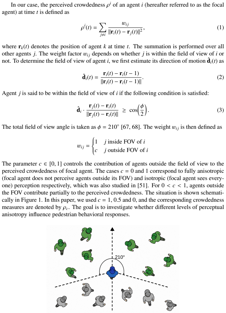
- Figure 1 caption and text: the FOV angle ϕ = 210° is taken from clinical perimetry literature; a brief note that results are expected to be robust to modest changes in ϕ (as with c) would be useful.
- Section 3: the weak correlation r ≲ 0.3 between δ1 and δ2 is reported with p-values; stating the exact sample size (or degrees of freedom) used for the correlation would improve transparency.
- Appendix A: the signed-deviation plots (Fig. 10) are helpful for interpreting the 30° early peaks; cross-referencing them more explicitly in the main-text discussion of α = 30° would aid readers who skip the appendix.
- Data/code availability: the Zenodo and GitHub links are welcome; ensuring the repository contains a short README that reproduces at least one main figure would further raise reproducibility standards.
Circularity Check
No significant circularity: empirical re-analysis of a public trajectory dataset with a literature-derived crowdedness index; qualitative robustness conclusions are not forced by construction of the measure or by self-citation.
full rationale
The paper defines a distance-weighted crowdedness index ho_c (Eq. 1) that incorporates a tunable FOV weight c otin {0, 0.5, 1} taken from the social-force literature and a fixed 210° FOV angle from clinical perimetry citations. It then applies this index, together with two directional-deviation angles and acceleration, to an independent public motion-capture dataset of crossing flows (Zenodo DOI given). All reported relationships (temporal profiles of ho, v– ho diagrams, ho– heta diagrams, a– ho diagrams, and non-retracing phase-space loops) are direct empirical averages over the trajectories; no free parameter is fitted to one subset of the data and then presented as a prediction of a related quantity. The interaction-window endpoints T_i, T_f used for the global time rescaling t' are inherited from the edge-cutting algorithm of the prior public release, but they are applied uniformly and the ho=0° baseline is handled separately; the rescaling does not algebraically force the observed geometry-versus-anisotropy ordering or the existence of the loops. Self-citations to the co-author’s earlier analyses of the same dataset supply context and the data themselves, yet the central claims (robustness of qualitative dynamics to c, smooth incremental turning, disruption–recovery asymmetry, superiority of dynamic fundamental diagrams) rest on the new multi-panel measurements rather than on an unverified uniqueness theorem or definitional identity. Consequently the derivation chain contains no self-definitional step, no fitted-input-as-prediction, and no load-bearing self-citation that collapses the result to its inputs.
Axiom & Free-Parameter Ledger
free parameters (4)
- FOV half-angle ϕ/2 =
210° total
- out-of-FOV weight c =
0, 0.5, 1
- turning window W =
0.5 s
- crowdedness bin width =
0.2 m^{-2}
axioms (3)
- ad hoc to paper Local interaction intensity is adequately captured by a sum of inverse-square distances weighted by a binary FOV indicator scaled by constant c.
- domain assumption The edge-cutting algorithm of Mullick et al. (2022) correctly identifies the temporal bounds of each crossing interaction.
- domain assumption Human visual field relevant to locomotion is 210°.
invented entities (1)
-
perceived crowdedness ρ_c
no independent evidence
read the original abstract
Pedestrian traffic is commonly characterized using local density, yet the interactions experienced by individuals depend on the relative positions and perceptual relevance of surrounding pedestrians. This raises the question of whether behavioral relationships inferred from local crowdedness are robust to the representation of perceptual anisotropy, and how interaction geometry shapes pedestrian adaptation over time. We analyze experimental pedestrian crossing flows over angles from 0 to 180 degrees using a distance-weighted measure of local crowdedness. Perceptual anisotropy is varied by reducing the contribution of pedestrians outside the focal pedestrian's field of view. We examine the temporal evolution of crowdedness and its relationships with velocity, directional deviation, and acceleration. Anisotropy primarily changes the numerical scale of crowdedness, while the qualitative dynamics, temporal progression, and crossing-angle dependence remain largely preserved. Pedestrians deviate appreciably from their expected group directions, but changes between successive walking directions remain small, indicating adaptation through smooth, incremental corrections rather than abrupt turns. Acceleration dynamics reveal an asymmetry between disruption and recovery: initial deceleration varies strongly with crossing geometry, whereas recovery accelerations are more similar across angles. Non-retracing trajectories in the behavioral phase spaces show that similar instantaneous conditions can correspond to different phases of the interaction. Overall, interaction geometry has a stronger influence on the organization of crossing flows than the perceptual weighting used to quantify local crowdedness. More broadly, dynamic fundamental diagrams provide a more complete characterization of transient pedestrian interactions than conventional relationships based on instantaneous state variables alone.
Figures


Reference graph
Works this paper leans on
-
[1]
Helbing, Reviews of modern physics73, 1067 (2001)
D. Helbing, Reviews of modern physics73, 1067 (2001)
2001
-
[2]
Schreckenberg, S.D
M. Schreckenberg, S.D. Sharma,Pedestrian and evacuation dynamics, V ol. 1 (Springer, 2002)
2002
-
[3]
Gibson, British journal of psychology49, 182 (1958)
J.J. Gibson, British journal of psychology49, 182 (1958)
1958
-
[4]
Batty, Nature388, 19 (1997)
M. Batty, Nature388, 19 (1997)
1997
-
[5]
Turner, A
A. Turner, A. Penn, Environment and planning B: Planning and Design29, 473 (2002)
2002
-
[6]
Gulikers, J
L. Gulikers, J. Evers, A. Muntean, A. Lyulin, Journal of Statistical Mechanics: Theory and Experiment2013, P04025 (2013)
2013
-
[7]
Wirth, G.C
T.D. Wirth, G.C. Dachner, K.W. Rio, W.H. Warren, PNAS nexus2, pgad118 (2023)
2023
-
[8]
Schrater, D.C
P.R. Schrater, D.C. Knill, E.P. Simoncelli, Nature neuroscience3, 64 (2000)
2000
-
[9]
Hopkins, A
B. Hopkins, A. Churchill, S. V ogt, L. Rönnqvist, Journal of motor behavior36, 3 (2004)
2004
-
[10]
Huber, Y .H
M. Huber, Y .H. Su, M. Krüger, K. Faschian, S. Glasauer, J. Hermsdörfer, PloS one9, e89589 (2014)
2014
-
[11]
Helbing,Social self-organization: Agent-based simulations and experiments to study emergent social behavior(Springer, 2012)
D. Helbing,Social self-organization: Agent-based simulations and experiments to study emergent social behavior(Springer, 2012)
2012
-
[12]
Moussaid, E.G
M. Moussaid, E.G. Guillot, M. Moreau, J. Fehrenbach, O. Chabiron, S. Lemercier, J. Pettré, C. Appert-Rolland, P. Degond, G. Theraulaz, PLoS computational biology8, e1002442 (2012)
2012
-
[13]
F. Gu, B. Guiselin, N. Bain, I. Zuriguel, D. Bartolo, Nature638, 112 (2025)
2025
-
[14]
Helbing, L
D. Helbing, L. Buzna, A. Johansson, T. Werner, Transportation science39, 1 (2005)
2005
-
[15]
Feliciani, K
C. Feliciani, K. Nishinari, Physical Review E94, 032304 (2016)
2016
-
[16]
Murakami, C
H. Murakami, C. Feliciani, Y . Nishiyama, K. Nishinari, Science Advances7, eabe7758 (2021)
2021
-
[17]
Khelfa, R
B. Khelfa, R. Korbmacher, A. Schadschneider, A. Tordeux, Scientific reports12, 4768 (2022)
2022
-
[18]
Bacik, B.S
K.A. Bacik, B.S. Bacik, T. Rogers, Science379, 923 (2023)
2023
-
[19]
Mullick, S
P. Mullick, S. Fontaine, C. Appert-Rolland, A.H. Olivier, W.H. Warren, J. Pettré, PLoS computational biology18, e1010210 (2022)
2022
-
[20]
Zanlungo, C
F. Zanlungo, C. Feliciani, Z. Yücel, K. Nishinari, T. Kanda, Safety science158, 105953 (2023)
2023
-
[21]
Zanlungo, C
F. Zanlungo, C. Feliciani, Z. Yücel, K. Nishinari, T. Kanda, Safety science158, 105969 (2023)
2023
-
[22]
Hoogendoorn, W
S.P. Hoogendoorn, W. Daamen, Transportation science39, 147 (2005)
2005
-
[23]
Seyfried, O
A. Seyfried, O. Passon, B. Steffen, M. Boltes, T. Rupprecht, W. Klingsch, Transporta- tion science43, 395 (2009)
2009
-
[24]
Zhang, W
J. Zhang, W. Klingsch, A. Schadschneider, A. Seyfried, inTraffic and Granular Flow’11 (Springer, 2013), pp. 241–249
2013
-
[25]
Moussaïd, D
M. Moussaïd, D. Helbing, G. Theraulaz, Proceedings of the National Academy of Sci- ences108, 6884 (2011)
2011
-
[26]
Dachner, T.D
G.C. Dachner, T.D. Wirth, E. Richmond, W.H. Warren, Proceedings of the Royal Soci- ety B: Biological Sciences289, 20212089 (2022)
2022
-
[27]
Corbetta, F
A. Corbetta, F. Toschi, Annual Review of Condensed Matter Physics14, 311 (2023)
2023
-
[28]
Dogbe, Journal of Mathematical Analysis and Applications387, 512 (2012)
C. Dogbe, Journal of Mathematical Analysis and Applications387, 512 (2012)
2012
-
[29]
Duives, W
D.C. Duives, W. Daamen, S.P. Hoogendoorn, Transportation Research Part C: Emerging Technologies37, 193 (2013)
2013
-
[30]
Van Toll, J
W. Van Toll, J. Pettré,Algorithms for microscopic crowd simulation: Advancements in the 2010s, inComputer Graphics Forum(Wiley Online Library, 2021), V ol. 40, pp. 731–754
2021
-
[31]
Korbmacher, A
R. Korbmacher, A. Nicolas, A. Tordeux, C. Totzeck, Crowd Dynamics, V olume 4: An- alytics and Human Factors in Crowd Modeling pp. 55–80 (2023)
2023
-
[32]
Helbing, P
D. Helbing, P. Molnar, Physical review E51, 4282 (1995)
1995
-
[33]
Burstedde, K
C. Burstedde, K. Klauck, A. Schadschneider, J. Zittartz, Physica A: Statistical Mechan- ics and its Applications295, 507 (2001)
2001
-
[34]
Vicsek, A
T. Vicsek, A. Czirók, E. Ben-Jacob, I. Cohen, O. Shochet, Physical review letters75, 1226 (1995)
1995
-
[35]
Kim, S.J
S. Kim, S.J. Guy, K. Hillesland, B. Zafar, A.A.A. Gutub, D. Manocha, The Visual Computer31, 541 (2015)
2015
-
[36]
Q. Xu, M. Chraibi, A. Seyfried, Transportation research part C: emerging technologies 133, 103464 (2021)
2021
-
[37]
Ond ˇrej, J
J. Ond ˇrej, J. Pettré, A.H. Olivier, S. Donikian, ACM Transactions on Graphics (TOG) 29, 1 (2010)
2010
-
[38]
Hoogendoorn, F.L
S.P. Hoogendoorn, F.L. van Wageningen-Kessels, W. Daamen, D.C. Duives, Physica A: Statistical Mechanics and its Applications416, 684 (2014)
2014
-
[39]
W.L. Koh, S. Zhou, ACM Transactions on Modeling and Computer Simulation (TOMACS)21, 1 (2011)
2011
-
[40]
Dietrich, G
F. Dietrich, G. Köster, Physical Review E89, 062801 (2014)
2014
-
[41]
Y . Xiao, Z. Gao, Y . Qu, X. Li, Transportation research part C: emerging technologies 68, 566 (2016)
2016
-
[42]
Helbing, I.J
D. Helbing, I.J. Farkas, T. Vicsek, inThe science of disasters: Climate disruptions, heart attacks, and market crashes(Springer, 2002), pp. 330–350
2002
-
[43]
Helbing, A
D. Helbing, A. Johansson, H.Z. Al-Abideen, Physical Review E—Statistical, Nonlinear, and Soft Matter Physics75, 046109 (2007)
2007
-
[44]
Helbing, P
D. Helbing, P. Mukerji, EPJ Data Science1, 7 (2012)
2012
-
[45]
Haghani, M
M. Haghani, M. Sarvi, Transportation Research Part B: Methodological107, 253 (2018)
2018
-
[46]
Feliciani, K
C. Feliciani, K. Shimura, K. Nishinari,Introduction to crowd management: Managing crowds in the digital era: Theory and Practice(Springer Nature, 2022)
2022
-
[47]
Feliciani, A
C. Feliciani, A. Corbetta, M. Haghani, K. Nishinari, Safety science164, 106174 (2023)
2023
-
[48]
Steffen, A
B. Steffen, A. Seyfried, Physica A: Statistical Mechanics and its Applications389, 1902 (2010)
1902
-
[49]
Schauer, M
L. Schauer, M. Werner, P. Marcus,Estimating crowd densities and pedestrian flows us- ing wi-fi and bluetooth, inProceedings of the 11th International Conference on Mobile and Ubiquitous Systems: Computing, Networking and Services(2014), pp. 171–177
2014
-
[50]
M. Wirz, T. Franke, D. Roggen, E. Mitleton-Kelly, P. Lukowicz, G. Tröster, EPJ Data Science2, 5 (2013)
2013
-
[51]
Duives, W
D.C. Duives, W. Daamen, S.P. Hoogendoorn, Physica A: Statistical Mechanics and its Applications427, 162 (2015)
2015
-
[52]
Tordeux, J
A. Tordeux, J. Zhang, B. Steffen, A. Seyfried, Journal of Statistical Mechanics: Theory and Experiment p. P06030 (2015)
2015
-
[53]
A.S. Rao, J. Gubbi, S. Marusic, M. Palaniswami, The Visual Computer31, 1533 (2015)
2015
-
[54]
Nagao, D
K. Nagao, D. Yanagisawa, K. Nishinari, Physica A: Statistical Mechanics and its Ap- plications510, 145 (2018)
2018
-
[55]
X. Ding, F. He, Z. Lin, Y . Wang, H. Guo, Y . Huang, IEEE Transactions on Intelligent Transportation Systems22, 4776 (2020)
2020
-
[56]
J. Wang, W. Lv, H. Jiang, Z. Fang, J. Ma, Transportation Research Part C: Emerging Technologies157, 104400 (2023)
2023
-
[57]
Mullick, C
P. Mullick, C. Appert-Rolland, W.H. Warren, J. Pettré, Physica A: Statistical Mechanics and its Applications657, 130251 (2025)
2025
-
[58]
Seyfried, B
A. Seyfried, B. Steffen, W. Klingsch, M. Boltes, Journal of Statistical Mechanics: The- ory and Experiment p. P10002 (2005)
2005
-
[59]
Geroliminis, C.F
N. Geroliminis, C.F. Daganzo, Transportation Research Part B: Methodological42, 759 (2008)
2008
-
[60]
Keyvan-Ekbatani, A
M. Keyvan-Ekbatani, A. Kouvelas, I. Papamichail, M. Papageorgiou, Transportation Research Part B: Methodological46, 1393 (2012)
2012
-
[61]
Paetzke, M
S. Paetzke, M. Boltes, A. Seyfried, Physica A: Statistical Mechanics and its Applica- tions595, 127077 (2022)
2022
-
[62]
Mullick, Transportation Science59, 990 (2025)
P. Mullick, Transportation Science59, 990 (2025)
2025
-
[63]
Cordes, A
J. Cordes, A. Nicolas, A. Schadschneider, Collective Dynamics9, 1 (2024)
2024
-
[64]
Cordes, A
J. Cordes, A. Schadschneider, A. Nicolas, PNAS nexus3, pgae120 (2024)
2024
-
[65]
García, D
A. García, D. Hernández-Delfin, D.J. Lee, M. Ellero, Physica A: Statistical Mechanics and its Applications612, 128461 (2023)
2023
-
[66]
Appert-Rolland, J
C. Appert-Rolland, J. Pettré, A.H. Olivier, W. Warren, A. Duigou-Majumdar, E. Pin- sard, A. Nicolas, Collective Dynamics5, 1–8 (2020)
2020
-
[67]
Traquair,An introduction to clinical perimetry(Kimpton, 1927)
H.M. Traquair,An introduction to clinical perimetry(Kimpton, 1927)
1927
-
[68]
H. Strasburger, i-Perception11, 2041669520913052 (2020) A Appendix: Interpretation of the initial deviation peaks forα=30 ◦ A distinct early-time behavior is observed for the shallow crossing angleα=30 ◦. In the plots of the mean absolute deviations (shown in Figure 5 of the main text), both⟨|δ 1|⟩and ⟨|δ2|⟩exhibit pronounced peaks during the initial part...
2020
discussion (0)
Sign in with ORCID, Apple, or X to comment. Anyone can read and Pith papers without signing in.