REVIEW 3 major objections 4 minor 33 references
Stable scalarized multi-horizon black holes exist only inside a window of primary scalar charge.
Reviewed by Pith at T0; open to challenge. T0 means a machine referee read the full paper against a public rubric. the ladder, T0–T4 →
T0 review · grok-4.5
2026-07-14 10:27 UTC pith:XMKUDZRK
load-bearing objection Solid multi-horizon extension of EEHS scalarization that produces a clean intermediate qs window for L/C branches, but the window rests on a radial s-mode time-domain proxy and an ADM-mass cut whose necessity is not fully argued. the 3 major comments →
Scalarization of Einstein-Euler-Heisenberg black hole with multiple horizons
The pith
A machine-rendered reading of the paper's core claim, the machinery that carries it, and where it could break.
Core claim
In the multi-horizon regime of the Einstein-Euler-Heisenberg-scalar theory with quadratic Maxwell coupling, the fundamental branches of scalarized low-, cold-, and hot-horizon black holes are dynamically stable only above a critical primary scalar charge, while the low and cold families further require the scalar charge to remain below an upper bound set by positivity of the ADM mass; thus viable solutions live in an intermediate window (or a lower bound for the hot family).
What carries the argument
The time-domain evolution of the radial s-mode scalar perturbation on the scalarized background, together with the positivity cut on ADM mass as a function of primary scalar charge qs, which together carve out the intermediate window of viability.
Load-bearing premise
That radial s-mode time-domain decay plus positivity of ADM mass are enough to certify a black hole as physically viable, without controlling non-radial modes or full quasinormal spectra.
What would settle it
A computation of the full quasinormal spectrum (or a non-radial mode analysis) on the same scalarized low- or cold-horizon solutions that finds an unstable mode inside the claimed intermediate window of primary scalar charge.
Editorial analysis
A structured set of objections, weighed in public.
Referee Report
Summary. The paper studies spontaneous scalarization of magnetically charged Einstein-Euler-Heisenberg black holes that possess multiple horizons (low, cold, negative, hot) for M=1 and μ=0.03. A quadratic coupling g(φ)=1-αφ^{2} is introduced only to the Maxwell term. Onset analysis (sufficient condition I_i<0, WKB bounds, and static scalar clouds) indicates infinite branches for the low, cold and hot horizons; the three fundamental (n=0) branches are then constructed numerically. Positivity of the ADM mass M_i(q_s) supplies upper bounds on primary scalar charge for the low and cold families, while time-domain evolution of a radial s-mode Gaussian packet under the Schrödinger-type equation with potential V_{s,i} shows that instabilities appear only at small q_s. The authors conclude that stable, physically viable scalarized solutions occupy an intermediate window of q_s for low/cold horizons and a lower bound for the hot horizon.
Significance. The multi-horizon EEHBH geometry (μ≤0.08) is a natural but previously unexplored arena for charge-induced scalarization. The numerical construction of three distinct fundamental branches, the mass-positivity cut that truncates the large-q_s tails of the L and C families, and the time-domain maps that reveal an unstable-to-stable transition within each fundamental branch are new results relative to the authors’ earlier single-horizon studies. If the intermediate-window claim survives more complete stability tests, it supplies a concrete, falsifiable prediction for the allowed range of primary scalar charge in nonlinear-electrodynamics scalarization models.
major comments (3)
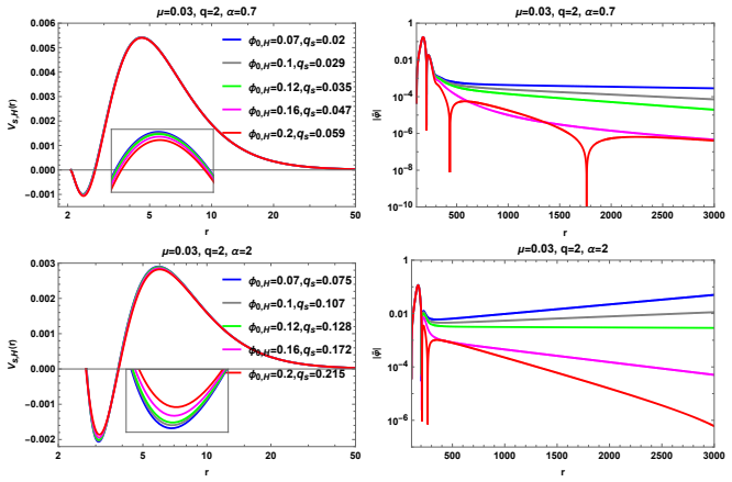
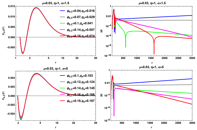
- §6, Eqs. (41)–(43) and Figs. 10–15: Dynamical stability of the fundamental branches is inferred solely from late-time decay of a radial (l=0) s-mode Gaussian packet. No complex QNM frequencies are extracted, non-radial multipoles are omitted, and metric/Maxwell perturbations are not coupled. The authors themselves note that the frequencies appear purely imaginary at small q_s and that full QNM extraction is “numerically challenging” (§6.3). Because the intermediate-window claim rests on this proxy, at least a partial QNM spectrum (or an explicit statement of its limitations) is required before the stability conclusion can be regarded as robust.
- §5, Fig. 8 and asymptotic expansion (37): The upper bounds q_s < q_s^u for the L and C branches are imposed by hand once the ADM mass M_i becomes negative. While M_i>0 is a natural physical requirement, the manuscript supplies no thermodynamic or asymptotic argument that negative-mass solutions must be discarded once the field equations and asymptotic flatness are already satisfied. Clarifying the status of this cut (or showing that other viability criteria independently exclude the same tail) is needed to keep the intermediate-window claim well-defined.
- §3 and Fig. 6: The WKB integrals that define α_in for the hot and negative horizons are declared “not properly defined” because f_i(r)<0 immediately outside those horizons. Consequently the cold horizon is adopted as the sole representative of the triple-horizon band. A more quantitative discussion of whether scalar clouds can still be constructed on the hot/negative backgrounds (or an explicit demonstration that they cannot) would strengthen the claim that only three families admit infinite branches.
minor comments (4)
- Notation for the four horizon families (r_L, r_C, r_N, r_H) is introduced in §2 but the thermodynamic labels “low/cold/negative/hot” are used interchangeably with the subscripts; a single consistent glossary would help the reader.
- Figs. 10–15 display many overlapping curves; a clearer legend or a tabular summary of the critical q_s values that separate unstable from stable regimes would improve readability.
- The coupling is restricted to the Maxwell term only; a brief remark on why the NED term F^{2} is left uncoupled (beyond the statement that it is the choice made) would be useful for comparison with Refs. [18,19].
- Several self-citations to the authors’ single-horizon EEHS papers appear; ensuring that the multi-horizon novelty is stated explicitly in the introduction would help the reader locate the new contribution.
Circularity Check
No significant circularity: multi-horizon scalarized solutions, mass bounds, and time-domain stability windows are independent numerical outputs from the EEHS equations, not forced by redefinition or self-citation chains.
full rationale
The derivation chain begins from the EEHS action (1) with quadratic coupling g(φ)=1-αφ^{2}, obtains the bald multi-horizon EEHBH metric (8) for µ=0.03, performs linearized onset analysis via the effective potential (20)–(22) and WKB/static eigenvalue problems to locate bifurcation points α_th, then constructs the n=0 scalarized branches by shooting the full nonlinear system (30)–(32) subject to asymptotic flatness (37). Upper bounds q_s^u on primary scalar charge follow directly from the numerical observation that ADM mass M_i(q_s) extracted from (37) becomes negative (Fig. 8); dynamical windows follow from time-domain integration of the radial s-mode Schrödinger equation (41) with potential (43). These are free-parameter numerical outputs (M=1, µ=0.03, q=0.5/1/2, α free). Self-citations to the authors’ single-horizon papers supply background methods and contrast, but the intermediate q_s windows themselves are not imported, fitted, or definitionally equivalent to any prior result. No uniqueness theorem, ansatz, or fitted constant is smuggled in as a prediction. The analysis is therefore self-contained against its own equations.
Axiom & Free-Parameter Ledger
free parameters (4)
- Euler-Heisenberg parameter μ
- Black-hole mass M
- Magnetic charges q (0.5, 1, 2)
- Coupling constants α_i and horizon scalars ϕ0,i
axioms (5)
- ad hoc to paper Einstein-Euler-Heisenberg-scalar action with g(ϕ)=1−αϕ² coupling only to the Maxwell term F, not to the NED F² term.
- domain assumption Spontaneous scalarization via tachyonic effective mass m²_eff=−α q²/r⁴ near the horizon with asymptotically vanishing scalar.
- domain assumption ADM mass positivity is required for physical viability of scalarized solutions.
- domain assumption Radial s-mode time-domain stability is a sufficient proxy for dynamical viability of the fundamental branches.
- standard math Asymptotically flat magnetically charged EEHBH metric (8) and standard thermodynamic definitions of T and horizon area.
invented entities (1)
-
Four named horizon families (low, cold, negative, hot) of the multi-horizon EEHBH
independent evidence
read the original abstract
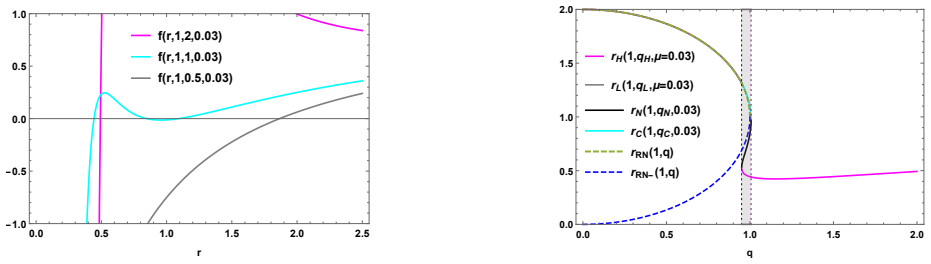
Scalarizations of the Einstein-Euler-Heisenberg (EEH) black hole (EEHBH) with multiple horizons are investigated in the EEH-scalar theory by introducing a quadratic scalar coupling to the Maxwell term. For mass $M=1$ and Euler-Heisenberg parameter $\mu=0.03$, the magnetically charged EEHBH admits four horizon families (low, cold, negative, and hot), with triple horizons appearing in the narrow band of magnetic charge $q\in[0.95,1.0065]$. The onset scalarization around the low, cold, and high horizons is then analyzed for the magnetic charge $q=0.5,\,1,\,2$, implying infinite branches of scalarized black holes for each case. We construct the three fundamental branches of scalarized black holes. From the positivity condition of their mass, we find the upper bounds on primary scalar charges $q_{s}$ for scalarized low and cold horizons. These bounds determine the allowable regions for the Hawking temperature and entropy. Furthermore, we perform a time-domain stability analysis and find that the instabilities arise only at small scalar charge regime. Therefore, stable and physically viable scalarized black holes exist in an intermediate window of the primary scalar charge for low and cold horizon solutions and a lower bound for hot horizon solution.
Figures





Reference graph
Works this paper leans on
-
[1]
R. Ruffini and J. A. Wheeler, Phys. Today24, no. 1, 30 (1971). doi:10.1063/1.3022513
-
[2]
J. D. Bekenstein, Phys. Rev. Lett.28, 452-455 (1972) doi:10.1103/PhysRevLett.28.452
-
[3]
J. D. Bekenstein, Phys. Rev. D5, 1239-1246 (1972) doi:10.1103/PhysRevD.5.1239
-
[4]
C. A. R. Herdeiro and E. Radu, Int. J. Mod. Phys. D24, no. 09, 1542014 (2015) doi:10.1142/S0218271815420146 [arXiv:1504.08209 [gr-qc]]
-
[5]
J. D. Bekenstein, Phys. Rev. D51, no.12, R6608 (1995) doi:10.1103/PhysRevD.51.R6608
-
[6]
D. D. Doneva and S. S. Yazadjiev, Phys. Rev. Lett.120, no.13, 131103 (2018) doi:10.1103/PhysRevLett.120.131103 [arXiv:1711.01187 [gr-qc]]
-
[7]
H. O. Silva, J. Sakstein, L. Gualtieri, T. P. Sotiriou and E. Berti, Phys. Rev. Lett.120, no.13, 131104 (2018) doi:10.1103/PhysRevLett.120.131104 [arXiv:1711.02080 [gr-qc]]
-
[8]
G. Antoniou, A. Bakopoulos and P. Kanti, Phys. Rev. Lett.120, no.13, 131102 (2018) doi:10.1103/PhysRevLett.120.131102 [arXiv:1711.03390 [hep-th]]
-
[9]
C. A. R. Herdeiro, E. Radu, N. Sanchis-Gual and J. A. Font, Phys. Rev. Lett.121, no.10, 101102 (2018) doi:10.1103/PhysRevLett.121.101102 [arXiv:1806.05190 [gr-qc]]
-
[10]
Y. S. Myung and D. C. Zou, Eur. Phys. J. C79, no.3, 273 (2019) doi:10.1140/epjc/s10052-019-6792-6 [arXiv:1808.02609 [gr-qc]]
-
[11]
W. Heisenberg and H. Euler, Z. Phys.98, no.11-12, 714-732 (1936) doi:10.1007/BF01343663 [arXiv:physics/0605038 [physics]]
-
[12]
Y. N. Obukhov and G. F. Rubilar, Phys. Rev. D66, 024042 (2002) doi:10.1103/PhysRevD.66.024042 [arXiv:gr-qc/0204028 [gr-qc]]
-
[13]
D. P. Sorokin, Fortsch. Phys.70(2022) no.7-8, 2200092 doi:10.1002/prop.202200092 [arXiv:2112.12118 [hep-th]]
-
[14]
H. Yajima and T. Tamaki, Phys. Rev. D63, 064007 (2001) doi:10.1103/PhysRevD.63.064007 [arXiv:gr-qc/0005016 [gr-qc]]. 26
-
[15]
Y. S. Myung, [arXiv:2503.18239 [gr-qc]]
-
[16]
T. Karakasis, G. Koutsoumbas, A. Machattou and E. Papantonopoulos, Phys. Rev. D106, no.10, 104006 (2022) doi:10.1103/PhysRevD.106.104006 [arXiv:2207.13146 [gr- qc]]
-
[17]
H. Guo, M. Park and Y. S. Myung, Chin. Phys. C50(2026) no.6, 065102 doi:10.1088/1674-1137/ae457c [arXiv:2508.16083 [gr-qc]]
-
[18]
L. Zhang, D. C. Zou and Y. S. Myung, Eur. Phys. J. C85, no.12, 1463 (2025) doi:10.1140/epjc/s10052-025-15232-4 [arXiv:2510.07954 [gr-qc]]
-
[19]
L. Zhang, Y. S. Myung, D. C. Zou and C. M. Zhang, [arXiv:2605.15566 [gr-qc]]
-
[20]
D. Amaro and A. Mac´ ıas, Phys. Rev. D102, no.10, 104054 (2020) doi:10.1103/PhysRevD.102.104054
-
[21]
N. Bret´ on and L. A. L´ opez, Phys. Rev. D104, no.2, 024064 (2021) doi:10.1103/PhysRevD.104.024064 [arXiv:2105.12283 [gr-qc]]
-
[22]
A. Allahyari, M. Khodadi, S. Vagnozzi and D. F. Mota, JCAP02, 003 (2020) doi:10.1088/1475-7516/2020/02/003 [arXiv:1912.08231 [gr-qc]]
-
[23]
C. Gao, Phys. Rev. D104, no.6, 064038 (2021) doi:10.1103/PhysRevD.104.064038 [arXiv:2106.13486 [gr-qc]]
-
[24]
J. L. Bl´ azquez-Salcedo, C. A. R. Herdeiro, J. Kunz, A. M. Pombo and E. Radu, Phys. Lett. B806, 135493 (2020) doi:10.1016/j.physletb.2020.135493 [arXiv:2002.00963 [gr- qc]]
-
[25]
Quasinormal modes of hot, cold and bald Einstein-Maxwell-scalar black holes
J. Luis Bl´ azquez-Salcedo, C. A. R. Herdeiro, S. Kahlen, J. Kunz, A. M. Pombo and E. Radu, Eur. Phys. J. C81, no.2, 155 (2021) doi:10.1140/epjc/s10052-021-08952-w [arXiv:2008.11744 [gr-qc]]
work page internal anchor Pith review Pith/arXiv arXiv doi:10.1140/epjc/s10052-021-08952-w 2021
-
[26]
Z. Luo and J. Li, Chin. Phys. C46, no.8, 085107 (2022) doi:10.1088/1674-1137/ac6574
-
[27]
G. Dotti and R. J. Gleiser, Class. Quant. Grav.22, L1 (2005) doi:10.1088/0264- 9381/22/1/L01 [arXiv:gr-qc/0409005 [gr-qc]]. 27
-
[28]
S. Hod, Phys. Lett. B798(2019), 135025 doi:10.1016/j.physletb.2019.135025 [arXiv:2002.01948 [gr-qc]]
-
[29]
G. Guo, P. Wang, H. Wu and H. Yang, Eur. Phys. J. C81(2021) no.10, 864 doi:10.1140/epjc/s10052-021-09614-7 [arXiv:2102.04015 [gr-qc]]
-
[30]
J. L. Bl´ azquez-Salcedo, D. D. Doneva, J. Kunz and S. S. Yazadjiev, Phys. Rev. D98 (2018) no.8, 084011 doi:10.1103/PhysRevD.98.084011 [arXiv:1805.05755 [gr-qc]]
-
[31]
H. O. Silva, C. F. B. Macedo, T. P. Sotiriou, L. Gualtieri, J. Sakstein and E. Berti, Phys. Rev. D99(2019) no.6, 064011 doi:10.1103/PhysRevD.99.064011 [arXiv:1812.05590 [gr-qc]]
-
[32]
C. F. B. Macedo, J. Sakstein, E. Berti, L. Gualtieri, H. O. Silva and T. P. Sotiriou, Phys. Rev. D99(2019) no.10, 104041 doi:10.1103/PhysRevD.99.104041 [arXiv:1903.06784 [gr-qc]]
-
[33]
Y. S. Myung and D. C. Zou, Eur. Phys. J. C79(2019) no.8, 641 doi:10.1140/epjc/s10052-019-7176-7 [arXiv:1904.09864 [gr-qc]]. 28
discussion (0)
Sign in with ORCID, Apple, or X to comment. Anyone can read and Pith papers without signing in.