REVIEW 2 major objections 6 minor 61 references
A Dirichlet-process weight prior lets Gaussian-splat mixtures choose their own component count in closed form and match fixed-budget fits with far fewer Gaussians.
Reviewed by Pith at T0; open to challenge. T0 means a machine referee read the full paper against a public rubric. the ladder, T0–T4 →
T0 review · grok-4.5
2026-07-14 08:20 UTC pith:ANU25AQW
load-bearing objection Clean, honest nonparametric complexity control for VBGS-style splat fitting; the math and deconfounded experiments hold up, and the deliberate scope limits are stated clearly. the 2 major comments →
DP-Splat: Bayesian Nonparametric Complexity Control for Gaussian Splatting
The pith
A machine-rendered reading of the paper's core claim, the machinery that carries it, and where it could break.
Core claim
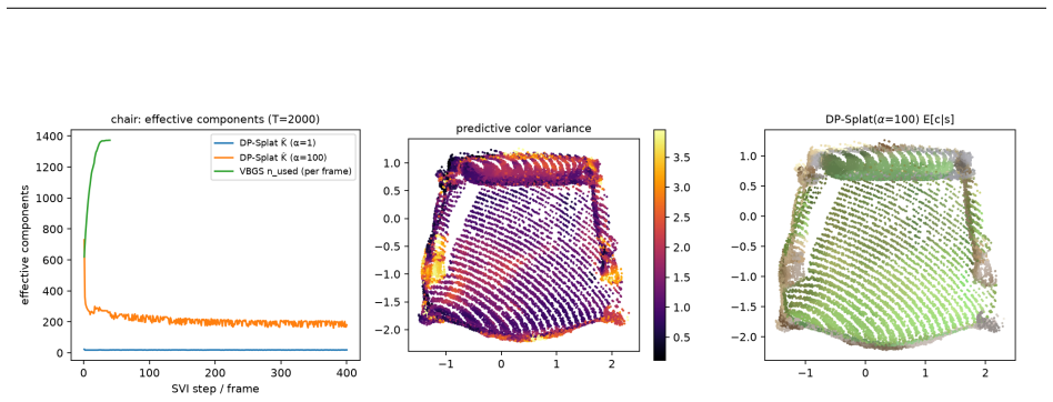
Switching only the mixture-weight prior of conjugate variational Gaussian splatting to a truncated stick-breaking Dirichlet process (or a sparse overfitted finite Dirichlet) makes the number of occupied components adapt to the data while preserving closed-form CAVI and SVI updates. The prior’s practical contribution is complexity selection, not better per-component efficiency: at matched effective budgets a converged Dirichlet-process fit ties a converged fixed-K fit, yet on 3D scenes it matches or exceeds the fixed-K baseline’s held-out color prediction with 5.9–7.6× fewer components. Under mean-field coordinate ascent at practical sample sizes the Dirichlet-process prior resists over-split
What carries the argument
The weight-prior switch: replace the finite symmetric Dirichlet over mixture weights with a truncated stick-breaking Dirichlet-process prior (primary) or a sparse overfitted Dirichlet (secondary), so Beta/Categorical/Normal–Inverse–Wishart (and optional Gamma) coordinate updates remain closed-form while the occupied-component count ˆK is an inference output.
Load-bearing premise
The whole argument rests on treating scene complexity as a mean-field mixture of colored points from depth-lifted RGB-D data, with coordinate ascent that permanently kills empty components and with rendering treated only as a downstream map that carries no guarantees.
What would settle it
On well-separated synthetic mixtures with known true K and a regime-appropriate fixed concentration, check whether recovered effective component count stays within ±1 of truth across N from 10^3 to 10^5; on the same 3D scene point clouds, check whether a single-pass Dirichlet-process fit at matched truncation still matches the fixed-K baseline’s held-out point-color PSNR while using several times fewer occupied components.
If this is right
- Scene fits can report an automatic effective Gaussian budget instead of requiring a user cap or densification heuristics.
- Held-out color prediction quality comparable to fixed large-K variational fits becomes available at roughly 6–8× fewer occupied components on the tested scenes.
- Posterior predictive color variance is available in closed form and is well calibrated when the generative model is correct.
- Truncation level T need only be a few times larger than the eventual ˆK; the corrected bound shows truncation error is negligible at typical scene budgets.
- Practitioners should not read ˆK as a consistent estimator of a true K; it is a pragmatic complexity control shaped by coordinate-ascent dynamics.
Where Pith is reading between the lines
- Uncertainty-aware next-best-view or densification could be driven directly by the closed-form Var[c|s] maps without extra networks.
- Adding merge/split or reordering moves would likely close the documented gap between variational ˆK growth and exact-posterior asymptotics.
- The same weight-prior switch could be dropped into other conjugate mixture scene models (e.g., continual SLAM variants) without redesigning the rest of the pipeline.
- If rasterized novel-view metrics track the point-level gains, automatic complexity control would become a practical alternative to post-hoc pruning of over-parameterized 3DGS models.
Editorial analysis
A structured set of objections, weighed in public.
Referee Report
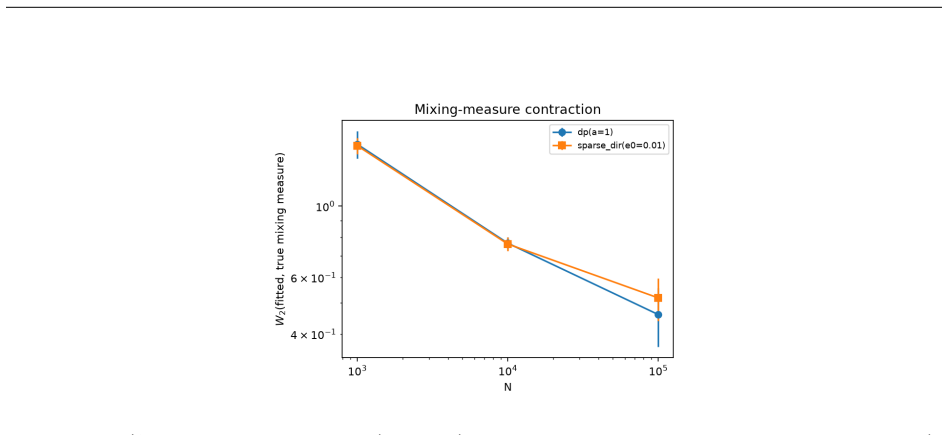
Summary. The paper replaces VBGS’s fixed-K finite Dirichlet weight prior with a truncated stick-breaking Dirichlet-process prior (primary) and a sparse overfitted finite Dirichlet (secondary), keeping the colored-point mixture fully conjugate so that CAVI and natural-gradient SVI remain closed-form. It supplies an exact ELBO monotonicity guarantee (Prop. 1), a rigorous finite-α truncation bound that corrects the commonly quoted anti-conservative large-α Ishwaran–James approximation (Prop. 2), and an explicit account of what the effective component count ˆK does and does not estimate under mean-field coordinate ascent. Empirically, ˆK recovers true K within ±1 on well-separated synthetics under regime-appropriate α; a deconfounded image comparison isolates the DP prior’s contribution to complexity selection rather than per-component efficiency (Table 1); on NeRF-synthetic RGB-D scenes DP-Splat matches or exceeds VBGS held-out point-color prediction with 5.9–7.6× fewer components; predictive color variance is well calibrated on model-matched data; and the paper documents a variational inversion of exact-posterior asymptotics across three orders of magnitude in N.
Significance. If the results hold as stated, this is a careful and useful bridge between classical Bayesian nonparametric mixture methodology and modern Gaussian-splatting scene representations. The contribution is deliberately statistical rather than leaderboard-oriented: closed-form nonparametric complexity control, a corrected truncation bound of practical relevance at the α regime these models use, calibrated posterior-predictive color variance, and a documented gap between variational practice and posterior asymptotics. Strengths that raise confidence include machine-checked update oracles, Monte-Carlo ELBO-term checks, cross-code regression against reference VBGS, multi-seed config-driven experiments with machine-readable records, and an unusually honest treatment of what ˆK estimates. These are genuine methodological assets for the community working on principled complexity control in splat-style models.
major comments (2)
- [§6.8, Table 2, Abstract] §6.8, Table 2, and the abstract’s 3D claim: the reported match/exceed of VBGS with 5.9–7.6× fewer components is on a rasterizer-free held-out point-color metric (E[c|s] on an unseen frame), not on novel-view rasterized PSNR/SSIM. The manuscript scopes this correctly in §3, §5 and §7, but the abstract and introduction still frame the work as complexity control for Gaussian Splatting practice. For the applied claim to land with a CV audience, either (i) add at least a limited rasterized quality-vs-budget comparison on the same fitted models, or (ii) rephrase the abstract/intro so that the 3D result is unambiguously a point-mixture predictive comparison, with rendering-grade evaluation deferred. As written, a reader can over-read the scene numbers as rendering results.
- [§6.2, Figure 2] §6.2 and Figure 2: recovery of K_true within ±1 requires a regime-appropriate fixed α (α=0.1 for K=3, α=1 for K=10, α=5 for K=30), and variational learning of α tracks the local optimum rather than correcting it. This is reported honestly, but it is load-bearing for the claim of automatic complexity control: without a usable α schedule or a merge/split/MFM mechanism, the practitioner still faces a concentration choice that plays a role analogous to choosing K. The paper should state more prominently (abstract or contributions list) that ˆK adaptation is automatic only conditional on a regime-appropriate concentration, and that learning α does not remove that requirement under plain CAVI.
minor comments (6)
- [§6.1, Figure 1] Figure 1 caption and §6.1: the 10% of DP seeds that land in visibly lower local optima are reported but not quantified in ELBO or ˆK terms. A one-line summary of the ELBO gap and resulting ˆK for those seeds would help readers assess practical risk.
- [Table 1] Table 1: the full-budget VBGS column is given only as a range (18.4–33.5 dB) while other columns report means and min/max. Adding a mean for the full-budget column would make the −6.47 / −4.79 dB gaps easier to interpret.
- [§4] §4, SVI paragraph: the schedule parameters (τ0=64, κsched=0.7, |B|=2^16) are stated without a short sensitivity note. Even a single sentence that conclusions are stable under modest schedule changes would strengthen the scaling claim.
- [§4, Effective complexity] Notation: n_min for the effective-component threshold and N_k for soft counts are easy to confuse on a first read; a brief reminder at first use of ˆK would help.
- [§2] Related work: BOGausS and PUP 3D-GS are cited; a one-sentence contrast with post-hoc pruning methods (that they act after a fixed-budget MLE fit, whereas DP-Splat builds parsimony into the prior) is already present but could be moved earlier for readers coming from the engineering compression line.
- [§4, Eq. (7)] Appendix E is thorough and useful; consider pointing to it more explicitly from Eq. (7) in the main text for readers who want the product-of-Student-t conditioning subtlety.
Circularity Check
No significant circularity: claims rest on classical conjugacy, stick-breaking, and external asymptotics, with empirical results not forced by definition or self-citation.
full rationale
The derivation chain is self-contained against external classical results and does not reduce predictions to fitted inputs by construction. Proposition 1 is standard conjugate mean-field CAVI monotonicity (Bishop §10.2). Proposition 2 derives a rigorous finite-α truncation bound from Ishwaran & James (2001) and corrects their large-α exponential approximation with an elementary inequality; the bound is not fitted to data. The predictive color moments (Eq. 7, Appendix E) follow from NIW conjugacy → Student-t (Murphy 2012) plus mean-field factorization and the law of total variance; they are verified against independent numerical integration, not against a fitted target. ˆK recovery on synthetics is explicitly conditioned on regime-appropriate fixed α and is reported as failing under a single α or under variational α-learning (mode-following); that is an honest empirical qualification, not a self-definitional loop. The deconfounded image comparison (Table 1) isolates complexity selection by tying against a converged fixed-K Dirichlet baseline at the same ˆK, so the +2.7 dB gap over single-pass VBGS is not re-labeled as a prior efficiency gain. Scene results use a priori α=100 and a rasterizer-free held-out point-color metric. Citations to Rousseau–Mengersen, Miller–Harrison, Nguyen, Blei–Jordan, Hoffman et al. are external classical literature; VBGS (Van de Maele et al.) is the baseline being modified, not a self-authored uniqueness theorem. Cross-code regression against the VBGS reference is verification, not load-bearing circular support. No step reduces a claimed prediction to its own inputs by construction.
Axiom & Free-Parameter Ledger
free parameters (6)
- DP concentration α (or Gamma hyper-parameters a0,b0 when learned)
- truncation level T
- sparse Dirichlet concentration e0
- effective-component threshold nmin
- NIW hyper-parameters (κ0=1e-3, ν0=Dm+2, Ψ0 from data variance)
- SVI schedule (τ0=64, κsched=0.7, |B|=2^16)
axioms (5)
- standard math Conjugacy of Normal–Inverse–Wishart, Beta, Categorical and Gamma families under the mean-field variational family yields exact coordinate-ascent maximizers of the ELBO.
- standard math The truncated stick-breaking construction with vT:=1 approximates the infinite DP with L1 error bounded by 2N(α/(1+α))^{T−1}.
- domain assumption Mean-field factorization q(π)∏k q(θk,s)q(θk,c) is an adequate variational family for the claims about ˆK, calibration and predictive moments.
- domain assumption The mixture density on colored points (RGB-D or depth-lifted) is the correct likelihood for complexity control; rasterized rendering is only a deployment map.
- ad hoc to paper Component death without revival under plain CAVI is an acceptable dynamics for pragmatic complexity control.
Cite this review
Pith. "Pith review of DP-Splat: Bayesian Nonparametric Complexity Control for Gaussian Splatting." pith.science (2026). https://pith.science/paper/ANU25AQW
@misc{pith2026260710912,
  author       = {Pith},
  title        = {Pith review of: DP-Splat: Bayesian Nonparametric Complexity Control for Gaussian Splatting},
  year         = {2026},
  howpublished = {\url{https://pith.science/paper/ANU25AQW}},
  note         = {Machine review of arXiv:2607.10912}
}
read the original abstract
3D Gaussian Splatting represents scenes as finite mixtures of anisotropic Gaussians whose number of components $K$ is set by heuristic density control or user caps. Variational Bayes Gaussian Splatting (VBGS) recast splat fitting as conjugate variational inference, but $K$ remains fixed. We replace the finite symmetric Dirichlet over mixture weights with a truncated stick-breaking Dirichlet-process prior -- and, as a theory-backed alternative, a sparse overfitted finite Dirichlet -- so that the number of occupied components adapts to the data while every update remains a closed-form coordinate-ascent step; a natural-gradient stochastic variant makes the per-step cost independent of the number of points. We give an exact monotonicity guarantee, a rigorous truncation-error bound correcting an anti-conservative large-$\alpha$ approximation in common use, and an honest account of what the fitted number of components estimates. Empirically: (i) the effective complexity $\hat{K}$ adapts to scene complexity and recovers the true $K$ within $\pm 1$ on well-separated synthetic data with regime-appropriate concentration; (ii) a deconfounded comparison shows the DP prior's contribution is complexity selection, not per-component efficiency -- converged DP fits exceed single-pass fixed-$K$ VBGS by +2.7 dB at matched budgets yet tie an equally converged fixed-$K$ baseline, and on 3D scenes DP-Splat matches or exceeds VBGS's held-out color prediction with 5.9-7.6x fewer components; (iii) the posterior-predictive color variance is well calibrated on model-matched synthetic data; and (iv) the ordering suggested by exact-posterior asymptotics reverses under mean-field coordinate ascent: the DP prior resists over-splitting while the sparse finite mixture saturates its truncation, a gap between variational practice and posterior asymptotics documented across three orders of magnitude in $N$.
Figures



Reference graph
Works this paper leans on
-
[1]
, title =
Ferguson, Thomas S. , title =. The Annals of Statistics , year =
-
[2]
Statistica Sinica , year =
Sethuraman, Jayaram , title =. Statistica Sinica , year =
-
[3]
, title =
Ishwaran, Hemant and James, Lancelot F. , title =. Journal of the American Statistical Association , year =
-
[4]
and Jordan, Michael I
Blei, David M. and Jordan, Michael I. , title =. Bayesian Analysis , year =
-
[5]
and Harrison, Matthew T
Miller, Jeffrey W. and Harrison, Matthew T. , title =. Advances in Neural Information Processing Systems , volume =. 2013 , publisher =
2013
-
[6]
and Harrison, Matthew T
Miller, Jeffrey W. and Harrison, Matthew T. , title =. Journal of Machine Learning Research , year =
-
[7]
and Harrison, Matthew T
Miller, Jeffrey W. and Harrison, Matthew T. , title =. Journal of the American Statistical Association , year =
-
[8]
Journal of the Royal Statistical Society: Series B (Statistical Methodology) , year =
Rousseau, Judith and Mengersen, Kerrie , title =. Journal of the Royal Statistical Society: Series B (Statistical Methodology) , year =
-
[9]
Model-Based Clustering Based on Sparse Finite
Malsiner-Walli, Gertraud and Fr. Model-Based Clustering Based on Sparse Finite. Statistics and Computing , year =
-
[10]
Generalized Mixtures of Finite Mixtures and Telescoping Sampling , journal =
Fr. Generalized Mixtures of Finite Mixtures and Telescoping Sampling , journal =. 2021 , volume =
2021
-
[11]
The Annals of Statistics , year =
Nguyen, XuanLong , title =. The Annals of Statistics , year =
-
[12]
Proceedings of the Twentieth International Joint Conference on Artificial Intelligence (
Kurihara, Kenichi and Welling, Max and Teh, Yee Whye , title =. Proceedings of the Twentieth International Joint Conference on Artificial Intelligence (. 2007 , pages =
2007
-
[13]
, title =
Bishop, Christopher M. , title =. 2006 , series =
2006
-
[14]
ACM Transactions on Graphics , volume =
Kerbl, Bernhard and Kopanas, Georgios and Leimk. ACM Transactions on Graphics , volume =. 2023 , doi =
2023
-
[16]
Advances in Neural Information Processing Systems , volume =
Kheradmand, Shakiba and Rebain, Daniel and Sharma, Gopal and Sun, Weiwei and Tseng, Yang-Che and Isack, Hossam and Kar, Abhishek and Tagliasacchi, Andrea and Yi, Kwang Moo , title =. Advances in Neural Information Processing Systems , volume =. 2024 , doi =
2024
-
[19]
and Tancik, Matthew and Barron, Jonathan T
Mildenhall, Ben and Srinivasan, Pratul P. and Tancik, Matthew and Barron, Jonathan T. and Ramamoorthi, Ravi and Ng, Ren , title =. Computer Vision -- ECCV 2020 , editor =. 2020 , doi =
2020
-
[20]
Advances in Neural Information Processing Systems , volume =
Fan, Zhiwen and Wang, Kevin and Wen, Kairun and Zhu, Zehao and Xu, Dejia and Wang, Zhangyang , title =. Advances in Neural Information Processing Systems , volume =. 2024 , doi =
2024
-
[21]
Proceedings of the IEEE/CVF Conference on Computer Vision and Pattern Recognition (CVPR) , pages =
Lee, Joo Chan and Rho, Daniel and Sun, Xiangyu and Ko, Jong Hwan and Park, Eunbyung , title =. Proceedings of the IEEE/CVF Conference on Computer Vision and Pattern Recognition (CVPR) , pages =
-
[22]
and Blei, David M
Hoffman, Matthew D. and Blei, David M. and Wang, Chong and Paisley, John , title =. Journal of Machine Learning Research , year =
-
[23]
and Kucukelbir, Alp and McAuliffe, Jon D
Blei, David M. and Kucukelbir, Alp and McAuliffe, Jon D. , title =. Journal of the American Statistical Association , year =
-
[24]
, title =
Murphy, Kevin P. , title =. 2012 , isbn =
2012
-
[25]
, title =
Ghahramani, Zoubin and Beal, Matthew J. , title =. Advances in Neural Information Processing Systems 12 , publisher =. 2000 , pages =
2000
-
[26]
Neural Computation , year =
Amari, Shun-ichi , title =. Neural Computation , year =
-
[27]
Proceedings of the 35th International Conference on Machine Learning , series =
Accurate Uncertainties for Deep Learning Using Calibrated Regression , author =. Proceedings of the 35th International Conference on Machine Learning , series =
-
[28]
Jiang, Wen and Lei, Boshu and Daniilidis, Kostas , booktitle =
-
[29]
Hanson, Alex and Tu, Allen and Singla, Vasu and Jayawardhana, Mayuka and Zwicker, Matthias and Goldstein, Tom , booktitle =
-
[30]
Le, Ya and Yang, Xuan , institution=. Tiny
-
[31]
On the Multivariate t Distribution , author=
-
[32]
The American Statistician , volume=
On the Conditional Distribution of the Multivariate t Distribution , author=. The American Statistician , volume=
-
[33]
Natural gradient works efficiently in learning
Shun-ichi Amari. Natural gradient works efficiently in learning. Neural Computation, 10 0 (2): 0 251--276, 1998. doi:10.1162/089976698300017746
-
[34]
Christopher M. Bishop. Pattern Recognition and Machine Learning. Information Science and Statistics. Springer, New York, 2006. ISBN 978-0-387-31073-2
2006
-
[35]
David M. Blei and Michael I. Jordan. Variational inference for D irichlet process mixtures. Bayesian Analysis, 1 0 (1): 0 121--143, 2006. doi:10.1214/06-BA104
doi:10.1214/06-ba104 2006
-
[36]
Blei, Alp Kucukelbir, and Jon D
David M. Blei, Alp Kucukelbir, and Jon D. McAuliffe. Variational inference: A review for statisticians. Journal of the American Statistical Association, 112 0 (518): 0 859--877, 2017. doi:10.1080/01621459.2017.1285773
-
[37]
On the conditional distribution of the multivariate t distribution
Peng Ding. On the conditional distribution of the multivariate t distribution. The American Statistician, 70 0 (3): 0 293--295, 2016
2016
-
[38]
LightGaussian : Unbounded 3D G aussian compression with 15x reduction and 200+ FPS
Zhiwen Fan, Kevin Wang, Kairun Wen, Zehao Zhu, Dejia Xu, and Zhangyang Wang. LightGaussian : Unbounded 3D G aussian compression with 15x reduction and 200+ FPS . In Advances in Neural Information Processing Systems, volume 37, pp.\ 140138--140158. Curran Associates, Inc., 2024. doi:10.52202/079017-4447
-
[39]
Thomas S. Ferguson. A B ayesian analysis of some nonparametric problems. The Annals of Statistics, 1 0 (2): 0 209--230, 1973. doi:10.1214/aos/1176342360
-
[40]
u hwirth-Schnatter, Gertraud Malsiner-Walli, and Bettina Gr \
Sylvia Fr \"u hwirth-Schnatter, Gertraud Malsiner-Walli, and Bettina Gr \"u n. Generalized mixtures of finite mixtures and telescoping sampling. Bayesian Analysis, 16 0 (4): 0 1279--1307, 2021. doi:10.1214/21-BA1294
-
[41]
Zoubin Ghahramani and Matthew J. Beal. Variational inference for B ayesian mixtures of factor analysers. In Advances in Neural Information Processing Systems 12, pp.\ 449--455. MIT Press, 2000
2000
-
[42]
PUP 3D-GS : Principled uncertainty pruning for 3D G aussian splatting
Alex Hanson, Allen Tu, Vasu Singla, Mayuka Jayawardhana, Matthias Zwicker, and Tom Goldstein. PUP 3D-GS : Principled uncertainty pruning for 3D G aussian splatting. In Proceedings of the IEEE/CVF Conference on Computer Vision and Pattern Recognition (CVPR), pp.\ 5949--5958, 2025
2025
-
[43]
Hoffman, David M
Matthew D. Hoffman, David M. Blei, Chong Wang, and John Paisley. Stochastic variational inference. Journal of Machine Learning Research, 14 0 (40): 0 1303--1347, 2013
2013
-
[44]
Hemant Ishwaran and Lancelot F. James. Gibbs sampling methods for stick-breaking priors. Journal of the American Statistical Association, 96 0 (453): 0 161--173, 2001. doi:10.1198/016214501750332758
-
[45]
FisherRF : Active view selection and mapping with radiance fields using F isher information
Wen Jiang, Boshu Lei, and Kostas Daniilidis. FisherRF : Active view selection and mapping with radiance fields using F isher information. In Computer Vision -- ECCV 2024, Lecture Notes in Computer Science, pp.\ 422--440. Springer, 2024
2024
-
[46]
3D G aussian splatting for real-time radiance field rendering
Bernhard Kerbl, Georgios Kopanas, Thomas Leimk \"u hler, and George Drettakis. 3D G aussian splatting for real-time radiance field rendering. ACM Transactions on Graphics, 42 0 (4): 0 1--14, July 2023. doi:10.1145/3592433
doi:10.1145/3592433 2023
-
[47]
3D G aussian splatting as M arkov chain M onte C arlo
Shakiba Kheradmand, Daniel Rebain, Gopal Sharma, Weiwei Sun, Yang-Che Tseng, Hossam Isack, Abhishek Kar, Andrea Tagliasacchi, and Kwang Moo Yi. 3D G aussian splatting as M arkov chain M onte C arlo. In Advances in Neural Information Processing Systems, volume 37, pp.\ 80965--80986. Curran Associates, Inc., 2024. doi:10.52202/079017-2573
-
[48]
Accurate uncertainties for deep learning using calibrated regression
Volodymyr Kuleshov, Nathan Fenner, and Stefano Ermon. Accurate uncertainties for deep learning using calibrated regression. In Proceedings of the 35th International Conference on Machine Learning, volume 80 of Proceedings of Machine Learning Research, pp.\ 2796--2804. PMLR, 2018
2018
-
[49]
Collapsed variational D irichlet process mixture models
Kenichi Kurihara, Max Welling, and Yee Whye Teh. Collapsed variational D irichlet process mixture models. In Proceedings of the Twentieth International Joint Conference on Artificial Intelligence ( IJCAI -07) , pp.\ 2796--2801, 2007
2007
-
[50]
Tiny ImageNet visual recognition challenge
Ya Le and Xuan Yang. Tiny ImageNet visual recognition challenge. Technical report, Stanford University, CS231N course report, 2015
2015
-
[51]
Compact 3D G aussian representation for radiance field
Joo Chan Lee, Daniel Rho, Xiangyu Sun, Jong Hwan Ko, and Eunbyung Park. Compact 3D G aussian representation for radiance field. In Proceedings of the IEEE/CVF Conference on Computer Vision and Pattern Recognition (CVPR), pp.\ 21719--21728, 2024
2024
-
[52]
u hwirth-Schnatter, and Bettina Gr \
Gertraud Malsiner-Walli, Sylvia Fr \"u hwirth-Schnatter, and Bettina Gr \"u n. Model-based clustering based on sparse finite G aussian mixtures. Statistics and Computing, 26 0 (1-2): 0 303--324, 2016. doi:10.1007/s11222-014-9500-2
-
[53]
Srinivasan, Matthew Tancik, Jonathan T
Ben Mildenhall, Pratul P. Srinivasan, Matthew Tancik, Jonathan T. Barron, Ravi Ramamoorthi, and Ren Ng. NeRF : Representing scenes as neural radiance fields for view synthesis. In Andrea Vedaldi, Horst Bischof, Thomas Brox, and Jan-Michael Frahm (eds.), Computer Vision -- ECCV 2020, volume 12346 of Lecture Notes in Computer Science, pp.\ 405--421. Springe...
-
[54]
Miller and Matthew T
Jeffrey W. Miller and Matthew T. Harrison. A simple example of D irichlet process mixture inconsistency for the number of components. In Advances in Neural Information Processing Systems, volume 26. Curran Associates, Inc., 2013
2013
-
[55]
Miller and Matthew T
Jeffrey W. Miller and Matthew T. Harrison. Inconsistency of P itman-- Y or process mixtures for the number of components. Journal of Machine Learning Research, 15: 0 3333--3370, 2014
2014
-
[56]
Jeffrey W. Miller and Matthew T. Harrison. Mixture models with a prior on the number of components. Journal of the American Statistical Association, 113 0 (521): 0 340--356, 2018. doi:10.1080/01621459.2016.1255636
-
[57]
Kevin P. Murphy. Machine Learning: A Probabilistic Perspective. MIT Press, Cambridge, MA, 2012. ISBN 978-0-262-01802-9
2012
-
[58]
Convergence of latent mixing measures in finite and infinite mixture models
XuanLong Nguyen. Convergence of latent mixing measures in finite and infinite mixture models. The Annals of Statistics, 41 0 (1): 0 370--400, 2013. doi:10.1214/12-AOS1065
-
[59]
BOGausS : Better optimized G aussian splatting
St \'e phane Pateux, Matthieu Gendrin, Luce Morin, Th \'e o Ladune, and Xiaoran Jiang. BOGausS : Better optimized G aussian splatting. arXiv preprint arXiv:2504.01844, 2025
Pith/arXiv arXiv 2025
-
[60]
On the multivariate t distribution
Michael Roth. On the multivariate t distribution. Technical Report LiTH-ISY-R-3059, Link \"o ping University, Division of Automatic Control, 2013
2013
-
[61]
Asymptotic behaviour of the posterior distribution in overfitted mixture models
Judith Rousseau and Kerrie Mengersen. Asymptotic behaviour of the posterior distribution in overfitted mixture models. Journal of the Royal Statistical Society: Series B (Statistical Methodology), 73 0 (5): 0 689--710, 2011. doi:10.1111/j.1467-9868.2011.00781.x
-
[62]
A constructive definition of D irichlet priors
Jayaram Sethuraman. A constructive definition of D irichlet priors. Statistica Sinica, 4 0 (2): 0 639--650, 1994
1994
-
[63]
Toon Van de Maele, Ozan C atal, Alexander Tschantz, Christopher L. Buckley, and Tim Verbelen. Variational B ayes G aussian splatting. arXiv preprint arXiv:2410.03592, 2024
arXiv 2024
-
[64]
VBGS-SLAM : Variational B ayesian G aussian splatting simultaneous localization and mapping
Yuhan Zhu, Yanyu Zhang, Jie Xu, and Wei Ren. VBGS-SLAM : Variational B ayesian G aussian splatting simultaneous localization and mapping. arXiv preprint arXiv:2604.02696, 2026
Pith/arXiv arXiv 2026
discussion (0)
Sign in with ORCID, Apple, or X to comment. Anyone can read and Pith papers without signing in.