REVIEW 3 major objections 5 minor
Antenna-level beam correction can erase mutual-coupling distortion inside a conditioned field of view, but sidelobes still spoil the EoR window unless the full sky is corrected.
Reviewed by Pith at T0; open to challenge. T0 means a machine referee read the full paper against a public rubric. the ladder, T0–T4 →
T0 review · grok-4.5
2026-07-14 05:35 UTC pith:EWKX6GLH
load-bearing objection Clean, simulation-backed voltage-to-visibility correction for mutual coupling that works inside a conditioned FoV and honestly shows why main-beam-only is not enough for EoR. the 3 major comments →
Direct Primary Beam Correction: Untangling Mutual Coupling in 21-cm Cosmological Experiments with the SKA-Low Radio Telescope
The pith
A machine-rendered reading of the paper's core claim, the machinery that carries it, and where it could break.
Core claim
Direct Primary Beam Correction reconstructs the far-field radiation pattern of a dense array down to the numerical noise floor inside a suitably conditioned field of view, and the same correction operator propagates unchanged from antenna voltages through beamforming into the visibility domain; yet main-beam-only application leaves chromatic grating-lobe power that continues to contaminate the EoR window, and the coupling imprint itself is temporally coherent and does not average down.
What carries the argument
Direct Primary Beam Correction: a regularised, direction-weighted linear inversion of stacked Jones (or array-pattern) matrices that maps embedded-element patterns onto an arbitrary reference pattern; the resulting matrix is applied once at the element level and carries through the entire signal chain by congruence.
Load-bearing premise
The embedded-element-pattern model used to build the correction matrix must be known to at least three significant figures across the sky; lower fidelity collapses the reconstruction.
What would settle it
Apply the same correction matrix to a real holographic or UAV-mapped beam set for an SKA-Low station and check whether residual power inside the conditioned field of view still falls below -80 dB and whether full-sky power spectra still show resonant leakage above the horizon limit.
If this is right
- Mutual-coupling mitigation can be performed in real time on antenna or beamformed voltages, or offline on visibilities, with no loss of accuracy and only O(M N_a^2) cost per channel.
- Main-beam-only correction strategies are unsafe for 21-cm power-spectrum experiments; full-sky correction or an explicit main-beam/sidelobe separation step is required before the delay transform.
- Because the coupling imprint is fixed by array geometry, longer integrations alone cannot suppress it; explicit modelling and correction remain mandatory.
- Correction-cycle artefacts average incoherently, so more frequent re-solving of the operator can reduce residual resonances at the price of compute.
- Reconstruction fidelity is set by three controllable knobs: Nyquist sky sampling, Tikhonov regularisation strength, and beam-model accuracy to three or more significant figures.
Where Pith is reading between the lines
- Holographic or satellite-beacon beam maps could replace simulated patterns inside the same operator, anchoring the correction to the as-built instrument rather than an idealised electromagnetic model.
- The same linear reconstruction could be pointed at any chosen reference pattern, not only the isolated element, offering a route to enforce a common station beam across an entire array.
- Combining the operator with image-domain apodisation or a tapered gridded estimator may suppress the residual sidelobe resonances without requiring a full-sky solve.
- If the three-significant-figure accuracy requirement cannot be met in the field, joint inference of beam parameters with the sky model may still be needed as a complementary path.
Editorial analysis
A structured set of objections, weighed in public.
Referee Report
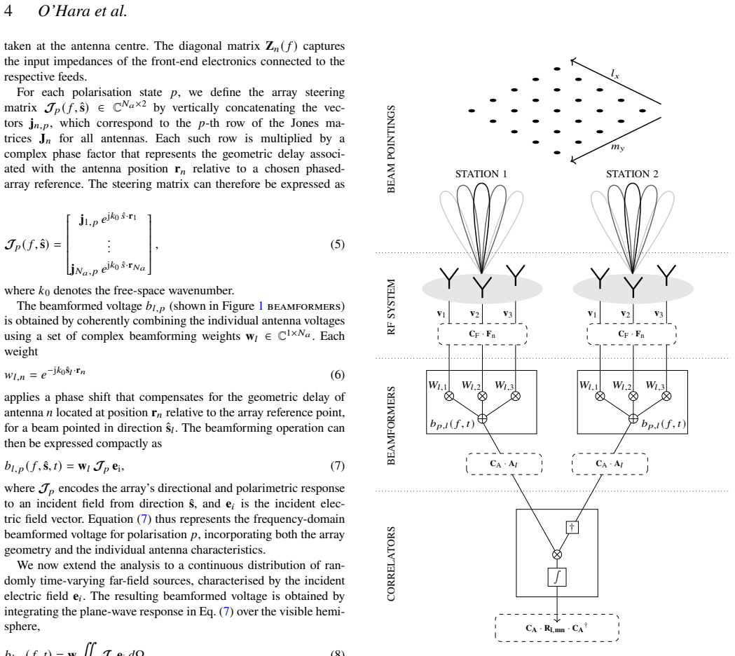
Summary. The paper introduces Direct Primary Beam Correction, a domain-agnostic framework that reconstructs an antenna far-field pattern toward an arbitrary reference by a regularised, direction-weighted linear inversion of stacked Jones matrices (Eqs. 22–24, 30). Applied to mutual coupling in dense aperture arrays, the operator maps embedded element patterns (EEPs) toward isolated element patterns (IEPs). Using full-wave FAST simulations of a perturbed Vogel SKA-Low station and OSKAR visibilities, the authors show that the operator reconstructs the pattern to the numerical noise floor inside a conditioned field of view (FoV), with fidelity set by Nyquist sampling, Tikhonov regularisation, and EEP model accuracy (§5.1–5.2, Figs. 3–5). The same operator propagates unchanged through beamformed voltages and visibilities via a congruence transformation (Eq. 32; Figs. 6–7). In a simulated 4-hour EoR0 observation (122–134 MHz), main-beam-only correction restores the EoR window, but full-sky sources through unconstrained sidelobes inject resonant, channel-incoherent contamination that can exceed the uncorrected EEP case (§6.1, Fig. 8). Coupling-induced leakage is temporally coherent and does not average down with integration time (§6.2, Figs. 9–10). The authors conclude that robust EoR recovery requires either full-sky correction or explicit main-beam/sidelobe separation before power-spectrum estimation.
Significance. If the result holds under realistic beam knowledge, the work supplies a computationally cheap, domain-agnostic route to mutual-coupling mitigation that can be applied at the voltage, beamformed, or visibility stage without recomputation. The formal equivalence between beamforming and interferometric imaging (Section 2) and the closed-form regularised inversion are cleanly derived and numerically verified with full-wave simulations. The science-facing diagnostics—main-beam success versus full-sky failure, and temporal coherence of coupling contamination—are directly relevant to SKA-Low and other dense 21-cm arrays, and the paper itself surfaces the load-bearing model-fidelity requirement (§5.2). Strengths include controlled residual maps to the numerical floor, explicit propagation tests, and power-spectrum diagnostics that falsify the naive “main-beam-only is enough” assumption.
major comments (3)
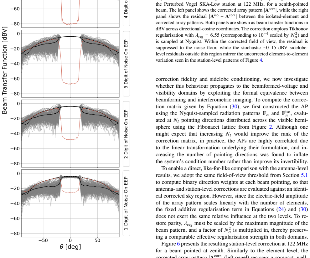
- [§5.2, Figs. 3–5] §5.2 and the abstract claim of reconstruction “down to the numerical noise floor”: the ideal residual floor (Figs. 3–4, <−80 dB) is obtained when the same simulated EEPs are used both to form the visibilities and to build C_F. The controlled noise test shows that two-significant-figure EEP accuracy already raises the residual floor to −45 to −50 dB and one-figure accuracy collapses the reconstruction. The central science claim therefore rests on an EEP model accurate to at least three (ideally four) significant figures across the sky. The manuscript should state this as an explicit operational requirement and discuss whether current holographic, UAV, or full-wave models meet it for SKA-Low, rather than leaving it as a sensitivity plot.
- [§6.1, Fig. 8] §6.1 (Fig. 8 bottom-right) and the abstract: main-beam-only correction is shown to be inadequate because unconstrained sidelobes inject resonant contamination that can exceed the uncorrected EEP. The paper correctly identifies the need for full-sky correction or main-beam/sidelobe separation, but offers only qualitative pointers (image apodisation, GPR, tapered gridded estimator) with no quantitative demonstration. Given that this is one of the two principal science implications, the manuscript should either (i) include a minimal demonstration that one of these strategies recovers the EoR window under the same simulation, or (ii) clearly reframe the claim as a diagnostic of the limitation rather than a completed mitigation path.
- [§3.1–3.2, Eqs. 24, 30] §3.1–3.2, Eqs. (24) and (30): Tikhonov λ_reg and the FoV cutoff (binary D) are free parameters that control the bias–variance trade-off. The adopted λ_reg = 10^−4 (and the N_a^2 rescaling at station level) is justified by residual maps, but there is no systematic scan of how residual power in the EoR window depends on these choices, nor a prescription for choosing them from data when the true IEP is unknown. A short robustness study or selection criterion would strengthen the claim that the framework is ready for deployment.
minor comments (5)
- [Fig. 2] Figure 2 caption: “red points (D=1)” and “red points (D=0)” appear to be a colour/label inconsistency; clarify which colour denotes included versus excluded directions.
- [§3] Notation: both F_n and f_n are used for element patterns; a single consistent symbol (and explicit statement that phase centres are included) would reduce ambiguity in §3.
- [§4.2] §4.2: the GSM is masked to a 5° radius while GLEAM is full-sky; a brief justification of why diffuse emission beyond 5° can be neglected while point sources cannot would help readers assess residual sky incompleteness.
- [§5.1] §5.1: the computational cost (2.94 s per channel) is useful; stating whether this is per station or per polarisation and how it scales with frequency across the full SKA-Low band would aid practical assessment.
- [References] References: several 2025–2026 citations (e.g. Abdurashidova et al. 2026, O’Hara et al. 2025b) are central; ensure final bibliographic details are complete at acceptance.
Circularity Check
Ideal-case reconstruction to the numerical noise floor is by construction from the same simulated EEPs used both to form the design matrix and to generate the ‘observed’ patterns/visibilities; the EoR-window and temporal-coherence claims remain independent diagnostics.
specific steps
-
self definitional
[§3.1 Eqs. 19–24; §5.1 Figs. 3–4; abstract]
"The relationship between the IEP and EEP for each element can be modelled as a linear transformation Fiso ≃ CF F … CF = Fiso D (FD)+ … we demonstrate that this framework reconstructs the radiation pattern down to the numerical noise floor within a suitably conditioned field of view"
CF is defined by least-squares as the operator that maps the stacked EEPs onto the IEP inside the support of D. When the identical noise-free EEPs that generate the mock data are also used to form the design matrix, the residual |Fiso – CF F| inside the FoV is zero (to machine precision) by construction of the pseudoinverse; the claimed ‘reconstruction to the numerical noise floor’ is therefore the definition of a successful fit, not an independent empirical result.
full rationale
The linear-algebra core (Eqs. 19–24, 27–30, 32) is ordinary weighted Tikhonov least-squares: CF (or CA) is defined as the map that sends the stacked EEPs onto the chosen reference (IEP) inside the support of D. When the identical, noise-free EEPs that generate the mock visibilities are also used to build CF, the residual inside the conditioned FoV necessarily saturates at the numerical floor of the pseudoinverse; this is self-definitional validation, not an independent prediction. The paper itself surfaces the limitation by injecting controlled complex Gaussian noise into the model EEPs (§5.2, Fig. 5) and showing monotonic degradation below three significant figures. The two principal science claims—main-beam-only correction leaves resonant sidelobe leakage that contaminates the EoR window (Fig. 8 bottom-right), and mutual-coupling contamination is temporally coherent across a 4-hour track (Figs. 9–10)—are obtained by applying the operator to full-sky GLEAM+GSM skies and do not reduce to the input model by construction. Self-citations (O’Hara et al. 2025, 2025b) supply only the shared simulation pipeline and prior evidence of coupling severity; they are not load-bearing uniqueness theorems. No cosmological parameters are fitted and then re-predicted. Overall circularity is therefore minor and confined to the perfect-model residual floor.
Axiom & Free-Parameter Ledger
free parameters (2)
- Tikhonov regularisation λ_reg =
10^{-4} (element), 6.55 (station)
- Correction FoV cutoff angle =
~16.2° at 122 MHz
axioms (4)
- domain assumption The radio interferometric measurement equation (RIME) correctly relates voltages, Jones matrices and sky brightness (Smirnov 2011).
- domain assumption Mutual coupling acts as a linear transformation between embedded and isolated element patterns (Huang et al. 2013).
- domain assumption Full-wave Method-of-Moments simulations (FAST) of the SKALA4 Perturbed Vogel station constitute ground-truth EEPs free of measurement noise.
- ad hoc to paper Tikhonov regularisation with a single scalar λ_reg sufficiently stabilises the under-constrained sidelobe modes without introducing unphysical spectral structure inside the FoV.
invented entities (1)
-
Direct Primary Beam Correction operator (C_F / C_A)
no independent evidence
read the original abstract
Mutual coupling between antennas has emerged as the dominant direction-dependent corruption in dense aperture arrays, imprinting pronounced sub-MHz spatial and spectral structure that compromises the time-gating and foreground-separation strategies used to isolate the faint 21-cm signal. In this work, we introduce \textit{Direct Primary Beam Correction}, a domain-agnostic framework for reconstructing the far-field radiation pattern relative to an arbitrary reference via a regularised, direction-weighted linear inversion of stacked Jones matrices, thereby enabling the removal of direction-dependent distortions such as mutual coupling. Using full-wave electromagnetic simulations of SKA-Low, we demonstrate that this framework reconstructs the radiation pattern down to the numerical noise floor within a suitably conditioned field of view, with the reconstruction accuracy governed by the regularised inversion and the fidelity of the underlying beam model. Applying the framework to a simulated 4-hour observation of the EoR0 field in the $122$--$134$~MHz band, we identify two principal implications for 21-cm power-spectrum analysis. First, restricting the correction to the main lobe and near sidelobes is inadequate: chromatic grating lobe contributions, whether left insufficiently or entirely uncorrected, continue to contaminate the EoR window. Second, mutual-coupling-induced contamination is temporally coherent and, being anchored to the fixed array geometry, does not average down across snapshots as the EoR field is tracked. Direct primary beam correction, therefore, provides a computationally efficient means of mitigating mutual coupling; however, robust recovery of the EoR window necessitates either full-sky correction or explicit separation of main-beam and sidelobe contributions prior to power-spectrum estimation.
Figures




discussion (0)
Sign in with ORCID, Apple, or X to comment. Anyone can read and Pith papers without signing in.