REVIEW 2 major objections 4 minor 38 references
A three-pulse composite sequence cancels the unknown-detuning bias in single-qubit Ramsey magnetometry to first order, removing the error floor that limits the single-pulse protocol.
Reviewed by Pith at T0; open to challenge. T0 means a machine referee read the full paper against a public rubric. the ladder, T0–T4 →
2026-08-02 05:11 UTC pith:VBYNA2GH
load-bearing objection A clean first-order fix for a systematic error floor in single-qubit Ramsey, with the residual higher-order gap honestly flagged; worth engaging despite the unquantified O(δ²) term. the 2 major comments →
Suppressing Detuning-Induced Bias in Ramsey Magnetometry with Composite Pulses
The pith
A machine-rendered reading of the paper's core claim, the machinery that carries it, and where it could break.
Core claim
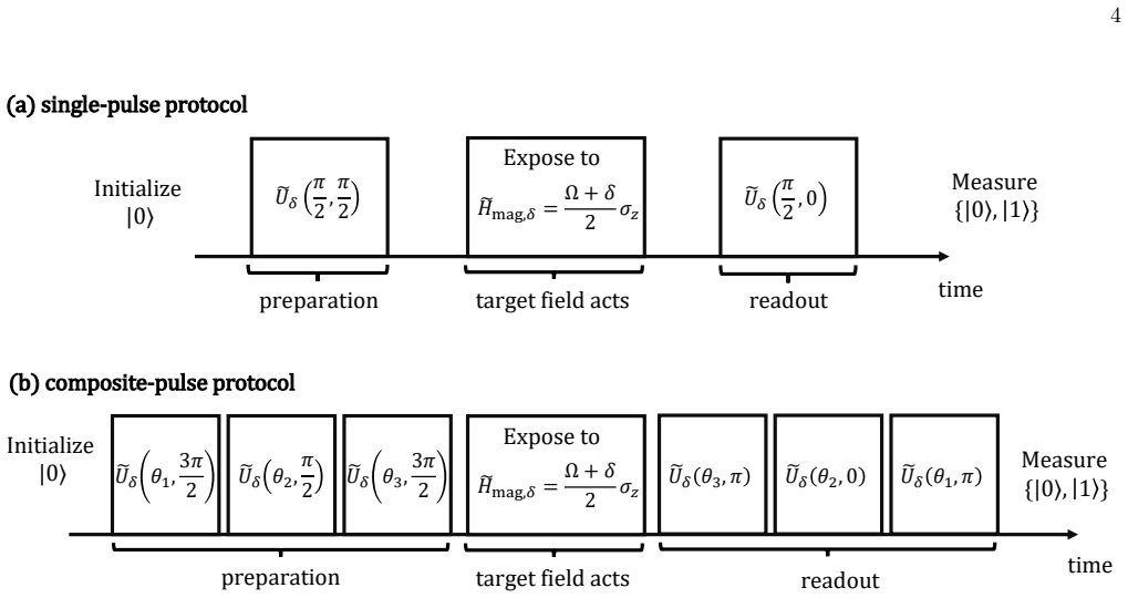
The paper's central claim is that the unknown-detuning bias in Ramsey magnetometry is a first-order systematic error that can be engineered away. In the single-pulse protocol, the first-order expansion U_δ(θ,φ) ≈ U(θ,φ) − iδ sin(θ/2) σ_z leads to an estimator bias b=(1+2/t)δ and a mean-square error floor b^2. The paper constructs a composite-pulse preparation, U_δ(θ3,3π/2) U_δ(θ2,π/2) U_δ(θ1,3π/2) with θ1=3π/4+A−B, θ2=2A, θ3=3π/4+A+B, A=arcsin(√(2α^2−2α+1)/(2√2)), B=arcsin(α/√(2α^2−2α+1)), α=t/4, and the corresponding reversed readout. These sequences make the first-order σ_z contributions from the pulses cancel the detuning term from the exposure, reducing the full protocol to the ideal dyn
What carries the argument
The central object is a three-pulse composite sequence—a short chain of rotations with carefully chosen angles and phases—that replaces each π/2 pulse. Starting from the first-order expansion of a detuned pulse, U_δ(θ,φ) ≈ U(θ,φ) − iδ sin(θ/2) σ_z, the paper shows the detuning error in each pulse acts as an extra σ_z rotation. The pulse areas θ1, θ2, θ3 are chosen, with α=t/4, so that these σ_z terms, together with the detuning phase accumulated during exposure, cancel to first order. This reduces the whole protocol to the ideal Ramsey dynamics plus O(δ^2). The mechanism relies on the fact that the target field acts only during exposure while the detuning acts throughout, which is what makes
Load-bearing premise
The central argument is perturbative in the detuning and assumes the rotating-wave approximation; the residual O(δ^2) bias is left unquantified, so the range of δ over which the cancellation is effective is not bounded.
What would settle it
Measure the outcome probability P_0 of the composite sequence versus detuning δ around δ=0 at fixed exposure time; Eq. (26) predicts a zero linear slope. A nonzero slope would falsify the first-order cancellation. Alternatively, compute the exact (non-perturbative) residual bias as a function of δ and check whether it exceeds the statistical error at the crossover δ*; if it does, the flat-error claim fails in the operating regime.
If this is right
- For detunings above the threshold δ*, the composite-pulse protocol achieves a smaller mean-square error than the single-pulse protocol; because δ* ∝ T^{-1/2}, longer experiments lower the threshold and widen the advantage.
- The composite protocol removes the detuning floor, so its error continues to decrease as total time T grows; the trade-off is a larger prefactor e^{2γτ_CP} due to the longer trial duration.
- The benefit holds under slowly drifting detunings: with block-wise random detuning, the composite error remains flat while the single-pulse error rises.
- Because the composite sequence acts on the control, it is complementary to data post-processing error-mitigation methods and can be combined with them.
- The derivation fixes the pulse areas from the exposure time t and requires t ≤ 2(1+√15) at λ=1, pinning the trial duration to τ_CP = t+7π; the paper analyzes this maximum-exposure configuration.
Where Pith is reading between the lines
- The first-order cancellation strategy could likely be extended to higher order in δ by lengthening the composite sequence and solving higher-order matching conditions; the paper does not attempt this and leaves the O(δ^2) residual unquantified.
- The same cancellation logic might apply to other coherent control imperfections that accumulate while the target field is off, such as pulse-amplitude miscalibration, although the specific pulse angles would need re-derivation.
- The threshold δ* ∝ T^{-1/2} suggests an adaptive protocol: run a short single-pulse survey to estimate δ, then switch to composite pulses if δ exceeds δ*; this would be a practical way to use the theoretical crossover.
- In configurations where the target field also acts during the pulses (e.g., continuous-wave sensing), the asymmetry the cancellation relies on disappears, so the composite construction would need to be modified; testing that variant would delimit the scheme's applicability.
Editorial analysis
A structured set of objections, weighed in public.
Referee Report
Summary. The paper analyzes systematic errors in single-qubit Ramsey magnetometry caused by an unknown detuning between the actual and nominal spin frequencies, with depolarizing noise. It first shows that a conventional single-pulse protocol incurs a detuning-induced bias b = (1 + 2/t)δ (Eq. 17), which produces a δ² floor in the mean-square error (Eq. 19). The authors then construct a composite-pulse preparation and readout (three pulses each, with explicit angles given in Eq. 24) that cancels the detuning to first order, exploiting the fact that the target field acts only during the exposure while the detuning acts throughout. The resulting protocol has mean-square error with no δ² floor to first order (Eq. 30), and a crossover threshold δ* versus the single-pulse protocol (Eq. 31). The analytical claims are supplemented by Monte Carlo simulations of the full (non-perturbative) dynamics, which show a flat composite-pulse RMS error in δ and a crossover near the predicted δ*.
Significance. If the result holds, the paper provides a control-level method to remove a specific systematic error in a basic quantum sensing protocol, complementing post-processing error-mitigation approaches. The derivation is clean and explicit: the composite pulse angles are derived from a first-order condition (Appendix B), and the Monte Carlo uses full dynamics, giving independent weight to the numerical claims. The authors are appropriately careful in stating that the cancellation is only to first order, and they explicitly flag in Section V that the residual second-order terms remain to be quantified. This honesty is a strength, but it also defines the main gap in the evidence.
major comments (2)
- [Sec. V / Eq. (26) / Eq. (30)] The central analytical claim that the composite-pulse protocol removes the detuning floor is established only to first order in δ. The outcome probability is given as P_CP = 1/2 + (1/2)e^{-γτ_CP} Ωt + O(δ²) (Eq. 26), and Eq. (30) then drops the O(δ²) term entirely. The threshold δ* of Eq. (31) likewise uses this first-order expression. Because the composite pulse areas are large (θ₂ = π, θ₁+θ₃ = 5π/2), the second-order coefficient could be substantial, and the manuscript provides no analytical estimate or bound. The Monte Carlo simulation of Fig. 2 demonstrates flatness for a specific parameter set (γ = 0.1, T = 2×10^8, δ up to 1.5×10^-3), which is helpful, but it does not replace an analytical characterization of the regime in which the first-order description is accurate. Please quantify the O(δ²) term (for example, derive its coefficient or provide a systematic numerical scan over γ,
- [Eq. (31)] The threshold δ* is presented as the condition for the composite protocol to outperform the single-pulse protocol. However, the square root in Eq. (31) is real only if the composite statistical term e^{2γτ_CP} τ_CP/(T t_CP²) exceeds the single-pulse term; otherwise no crossover exists and the composite protocol is never better. The manuscript does not state this condition or discuss the parameter regime (for example, large γ) where the composite protocol's longer duration makes it uncompetitive. This is a gap in the analytical trade-off and should be addressed, even if only by a brief comment.
minor comments (4)
- [Figs. 2 and 3] The y-axis tick labels appear as '10 4' and '10 3', which I interpret as 10^{-4} and 10^{-3}. Please typeset them as true superscripts for clarity.
- [Eq. (15)] The notation O(δ², Ω², Ωδ) is ambiguous; it would be clearer to write O(δ²) + O(Ω²) + O(Ωδ).
- [Sec. IV B] The Monte Carlo simulation states that the exact outcome probability P0 is computed from density-matrix evolution, but it does not specify how the exact propagators are obtained (e.g., matrix exponentials of the full Hamiltonian including detuning and RWA). A brief description would improve reproducibility.
- [References] Reference [19] is cited as a published PRA article with a 2026 date; if this is an in-press or preprint, consider adding the arXiv number or DOI to aid the reader.
Circularity Check
No significant circularity: the composite-pulse sequence is constructed from an explicit first-order matching condition and then tested against full non-perturbative Monte Carlo dynamics.
full rationale
The paper's central claim is that a specifically designed composite-pulse preparation and readout cancels the detuning-induced bias to first order in δ. This is not circular: the pulse areas θ1,θ2,θ3 are derived in Appendix B by solving the matching condition Eq. (B1), i.e., the sequence is constructed to produce the desired first-order term σ0+i(δt/4)σz. The subsequent claim that the bias is removed is the direct, acknowledged consequence of this construction, not a hidden reuse of the conclusion as an input. Crucially, the performance evaluation in Sec. IV B uses Monte Carlo sampling of the full non-perturbative density-matrix dynamics with independent binomial trials, so the flat RMS curve and the crossover near δ*≈7.5×10⁻⁴ are genuine numerical predictions rather than fits to the same data used to determine the pulse parameters. The analytical expressions Eq. (26) and Eq. (30) follow from the first-order calculation and are not obtained by renaming or refitting simulation output. The only same-author citation, Ref. [19], is background about detuning compensation in GHZ-based metrology and is not load-bearing for the single-qubit derivation; Appendix B is self-contained. The paper explicitly acknowledges at the end of Sec. V that 'the residual second-order terms remain to be quantified.' That is a limitation/robustness gap in the regime of validity of the first-order cancellation, but it is not a circular step: it does not make the first-order prediction equivalent to its input by construction. No self-definitional reduction, no fitted input relabeled as prediction, and no self-citation chain forces the central result.
Axiom & Free-Parameter Ledger
free parameters (5)
- Composite pulse angles theta_1, theta_2, theta_3 =
theta_1 = 3pi/4 + A - B, theta_2 = 2A, theta_3 = 3pi/4 + A + B
- Exposure time t_CP = 2(1+sqrt(15)) =
2(1+sqrt(15)) ~ 9.746
- Single-pulse optimal exposure t_SP =
t_SP = [1 - 2 gamma pi + sqrt(4 gamma^2 pi^2 + 12 gamma pi + 1)] / (4 gamma) ~ 6.611 at gamma=0.1
- Depolarizing rate gamma =
gamma = 0.1 in numerics
- Total experimental time T =
T = 2e8 in numerics
axioms (5)
- domain assumption Rotating-wave approximation: counter-rotating terms at 2 omega_0 are neglected, giving a correction of order Lambda/omega_0.
- domain assumption The drive is resonant with the nominal frequency, omega = omega_0.
- domain assumption Depolarizing noise is isotropic and acts independently on each trial, with a known rate gamma.
- domain assumption The field acts only during exposure, while detuning acts throughout the protocol.
- domain assumption The detuning delta is small; all analytic results are first-order in delta.
Cite this review
Pith. "Pith review of Suppressing Detuning-Induced Bias in Ramsey Magnetometry with Composite Pulses." pith.science (2026). https://pith.science/paper/VBYNA2GH
@misc{pith2026260713422,
  author       = {Pith},
  title        = {Pith review of: Suppressing Detuning-Induced Bias in Ramsey Magnetometry with Composite Pulses},
  year         = {2026},
  howpublished = {\url{https://pith.science/paper/VBYNA2GH}},
  note         = {Machine review of arXiv:2607.13422}
}
read the original abstract
Quantum sensing estimates a physical parameter encoded in the state of a probe; with independent spin probes the precision follows the standard quantum limit. Studies of sensing precision often assume that the parameters entering the model, such as the noise, are known. In practice these parameters are not always known, and a mismatch between the assumed and actual values induces a systematic error. Here we study single-qubit Ramsey magnetometry of a DC magnetic field under an unknown detuning between the actual and nominal spin frequencies: A first pulse puts the qubit into a superposition of its two states, the field to be sensed then adds a relative phase during an exposure stage, and a second pulse enables the readout. In our setting, the field acts only during the exposure stage, whereas the detuning acts throughout the whole protocol. We analyze how the detuning biases the estimate, preventing the total estimation error from following the standard quantum limit. We then construct a composite-pulse preparation and readout that exploits the difference in the intervals over which the field and the detuning act to cancel the detuning to first order. We evaluate the performance of this composite-pulse protocol and show that it suppresses the detuning-induced bias.
Figures

Reference graph
Works this paper leans on
-
[1]
The rescaling in Eq
The linear estimator remains unbiased,⟨ ˜Ω⟩= Ω. The rescaling in Eq. (7) carries a cost: it multiplies the ideal mean-square error of Eq. (4) bye 2γτ , EMS = ( ˜Ω−Ω) 2 ≈ e2γτ M t2 .(8) This prefactor is the cost of undoing the damping. It raises the error but leaves theO(M −1/2) scaling un- changed. This is unlike entanglement-enhanced metrol- ogy [32], w...
-
[2]
J. F. Barry, J. M. Schloss, E. Bauch, M. J. Turner, C. A. Hart, L. M. Pham, and R. L. Walsworth, Sensitivity optimization for nv-diamond magnetometry, Reviews of Modern Physics92, 015004 (2020)
2020
-
[3]
(C6) This givesτ CP =t CP + 7πatλ= 1, consistent with Eq. (27). The statistical term is then β e2γβt CP T t2 CP ,(C7) and its derivative vanishes at t∗ CP = 1 2βγ = 1 + √ 15 γ 2(1 + √
-
[4]
+ 7π ,(C8) corresponding toλ ∗ = 2γ 2(1 + √
-
[5]
This stationary point is a minimum, but the exposure must satisfyt CP ≥2(1 + √ 15), corresponding toλ≤1
+ 7π . This stationary point is a minimum, but the exposure must satisfyt CP ≥2(1 + √ 15), corresponding toλ≤1. Whent ∗ CP falls below this bound, the minimum over the allowed range is attained at the bound. The optimal exposure is therefore topt CP = max 1 + √ 15 γ 2(1 + √
-
[6]
Both protocols therefore useλ= 1 in the numerical study of Sec
+ 7π ,2(1 + √ 15) ! .(C9) At the valueγ= 0.1 used in the main text, the first argument is smaller than 2(1 + √ 15), so the optimum is topt CP = 2(1 + √ 15), attained atλ= 1. Both protocols therefore useλ= 1 in the numerical study of Sec. IV B
-
[7]
C. L. Degen, F. Reinhard, and P. Cappellaro, Quantum sensing, Reviews of Modern Physics89, 035002 (2017)
2017
-
[8]
Giovannetti, S
V. Giovannetti, S. Lloyd, and L. Maccone, Quantum- enhanced measurements: beating the standard quantum limit, Science306, 1330 (2004)
2004
-
[9]
Aslam, H
N. Aslam, H. Zhou, E. K. Urbach, M. J. Turner, R. L. Walsworth, M. D. Lukin, and H. Park, Quantum sensors for biomedical applications, Nature Reviews Physics5, 157 (2023)
2023
-
[10]
Montenegro, C
V. Montenegro, C. Mukhopadhyay, R. Yousefjani, S. Sarkar, U. Mishra, M. G. Paris, and A. Bayat, Quan- tum metrology and sensing with many-body systems, Physics Reports1134, 1 (2025)
2025
-
[11]
J. R. Maze, P. L. Stanwix, J. S. Hodges, S. Hong, J. M. Taylor, P. Cappellaro, L. Jiang, M. G. Dutt, E. Togan, A. Zibrov, et al., Nanoscale magnetic sensing with an individual electronic spin in diamond, Nature455, 644 (2008)
2008
-
[12]
J. M. Taylor, P. Cappellaro, L. Childress, L. Jiang, D. Budker, P. R. Hemmer, A. Yacoby, R. Walsworth, and M. D. Lukin, High-sensitivity diamond magnetometer with nanoscale resolution, Nature Physics4, 810 (2008)
2008
-
[13]
T. Wolf, P. Neumann, K. Nakamura, H. Sumiya, T. Ohshima, J. Isoya, and J. Wrachtrup, Subpicotesla diamond magnetometry, Physical Review X5, 041001 (2015)
2015
-
[14]
A. Shimada, H. Hakoshima, S. Endo, K. Yamamoto, and Y. Matsuzaki, Quantum sensing to suppress system- atic errors with measurements in the zeno regime, arXiv preprint arXiv:2103.14402 (2021)
Pith/arXiv arXiv 2021
-
[15]
The exposure scales ast CP = 2(1 + √ 15)/λ, and we optimize it by varyingλ
whenλ= 1, but we can tune this by changingλ. The exposure scales ast CP = 2(1 + √ 15)/λ, and we optimize it by varyingλ. Lowering λlengthens the exposure but also lengthens the control, making the optimization nontrivial. Asλ= 1 is the maximum, the exposure obeyst CP ≥2(1 + √ 15). The trial duration scales with it,τ CP =β tCP, where β= 2(1 + √
-
[16]
Huang, M
J. Huang, M. Zhuang, and C. Lee, Entanglement- enhanced quantum metrology: From standard quantum limit to heisenberg limit, Applied Physics Reviews11 (2024)
2024
-
[17]
Suzuki, Y
J. Suzuki, Y. Yang, and M. Hayashi, Quantum state es- timation with nuisance parameters, J. Phys. A: Math. Theor.53, 453001 (2020)
2020
-
[18]
Sugiyama, Precision-guaranteed quantum metrology, Physical Review A91, 042126 (2015)
T. Sugiyama, Precision-guaranteed quantum metrology, Physical Review A91, 042126 (2015)
2015
-
[19]
Takeuchi, Y
Y. Takeuchi, Y. Matsuzaki, K. Miyanishi, T. Sugiyama, and W. J. Munro, Quantum remote sensing with asym- metric information gain, Physical Review A99, 022325 (2019)
2019
-
[20]
S. Pang, J. R. G. Alonso, T. A. Brun, and A. N. Jordan, Protecting weak measurements against systematic errors, Physical Review A94, 012329 (2016). 9
2016
-
[21]
Yamamoto, S
K. Yamamoto, S. Endo, H. Hakoshima, Y. Matsuzaki, and Y. Tokunaga, Error-mitigated quantum metrology via virtual purification, Phys. Rev. Lett.129, 250503 (2022)
2022
-
[22]
H. Kwon, C. Oh, Y. Lim, H. Jeong, and L. Jiang, Efficacy of virtual purification-based error mitigation on quantum metrology, Phys. Rev. A109, 022410 (2024)
2024
-
[23]
H. Kwon, C. Oh, Y. Lim, H. Jeong, S.-W. Lee, and L. Jiang, Virtual purification complements quantum er- ror correction in quantum metrology, arXiv preprint arXiv:2503.12614 (2025)
Pith/arXiv arXiv 2025
-
[24]
Lin and H
X. Lin and H. Yuan, Error-mitigated quantum metrol- ogy via enhanced virtual purification, Communications Physics8, 481 (2025)
2025
-
[25]
Kukita and Y
S. Kukita and Y. Matsuzaki, Mitigating detuning- induced systematic errors in entanglement-enhanced metrology, Phys. Rev. A113, 042414 (2026)
2026
-
[26]
Tanaka, P
T. Tanaka, P. Knott, Y. Matsuzaki, S. Dooley, H. Ya- maguchi, W. J. Munro, and S. Saito, Proposed robust entanglement-based magnetic field sensor beyond the standard quantum limit, Phys. Rev. Lett.115, 170801 (2015)
2015
-
[27]
J. A. Jones, S. D. Karlen, J. Fitzsimons, A. Ardavan, S. C. Benjamin, G. A. D. Briggs, and J. J. Morton, Mag- netic field sensing beyond the standard quantum limit using 10-spin noon states, science324, 1166 (2009)
2009
-
[28]
M. H. Levitt, Composite pulses, Progress in Nuclear Magnetic Resonance Spectroscopy18, 61 (1986)
1986
-
[29]
Counsell, M
C. Counsell, M. Levitt, and R. Ernst, Analytical theory of composite pulses, Journal of Magnetic Resonance (1969) 63, 133 (1985)
1969
-
[30]
H. K. Cummins, G. Llewellyn, and J. A. Jones, Tackling systematic errors in quantum logic gates with composite rotations, Phys. Rev. A67, 042308 (2003)
2003
-
[31]
Levitt, Spin Dynamics: Basics of Nuclear Magnetic Resonance (Wiley, 2008)
M. Levitt, Spin Dynamics: Basics of Nuclear Magnetic Resonance (Wiley, 2008)
2008
-
[32]
Timoney, V
N. Timoney, V. Elman, S. Glaser, C. Weiss, M. Johan- ning, W. Neuhauser, and C. Wunderlich, Error-resistant single-qubit gates with trapped ions, Phys. Rev. A77, 052334 (2008)
2008
-
[33]
H. Ball, M. J. Biercuk, A. R. R. Carvalho, J. Chen, M. Hush, L. A. De Castro, L. Li, P. J. Liebermann, H. J. Slatyer, C. Edmunds, V. Frey, C. Hempel, and A. Milne, Software tools for quantum control: improving quantum computer performance through noise and error suppres- sion, Quantum Science and Technology6, 044011 (2021)
2021
-
[34]
Zanon-Willette, R
T. Zanon-Willette, R. Lefevre, R. Metzdorff, N. Silli- toe, S. Almonacil, M. Minissale, E. de Clercq, A. V. Taichenachev, V. I. Yudin, and E. Arimondo, Compos- ite laser-pulses spectroscopy for high-accuracy optical clocks: a review of recent progress and perspectives, Re- ports on Progress in Physics81, 094401 (2018)
2018
-
[35]
D. M. Lancaster, M. A. Shahbaz, H. G. Yousefabad, S. Chatterjee, E. Ram, and J. D. Weinstein, Quantum sensing in the presence of pulse errors and qubit leakage, arXiv preprint arXiv:2509.09874 (2025)
Pith/arXiv arXiv 2025
-
[36]
C. D. Aiello, M. Hirose, and P. Cappellaro, Composite- pulse magnetometry with a solid-state quantum sensor, Nat. Commun.4, 1419 (2013)
2013
-
[37]
N. F. Ramsey, A molecular beam resonance method with separated oscillating fields, Phys. Rev.78, 695 (1950)
1950
-
[38]
S. F. Huelga, C. Macchiavello, T. Pellizzari, A. K. Ekert, M. B. Plenio, and J. I. Cirac, Improvement of frequency standards with quantum entanglement, Physical Review Letters79, 3865 (1997)
1997
This paper was first reviewed by deepseek-v4-flash on August 2, 2026.
discussion (0)
Sign in with ORCID, Apple, or X to comment. Anyone can read and Pith papers without signing in.