REVIEW 4 major objections 6 minor 153 references
For the image benchmarks studied, a Quantum Extreme Learning Machine reaches its full accuracy once local entanglement has built up over a finite range, at a timescale independent of system size; from then on its performance equals that of
Reviewed by Pith at T0; open to challenge. T0 means a machine referee read the full paper against a public rubric. the ladder, T0–T4 →
T0 review · deepseek-v4-flash
2026-08-02 04:01 UTC pith:JQUEJZ4I
load-bearing objection A coherent thesis compiling two published QELM papers; the new material is a preliminary QELM-on-neutrino pilot, and the core claim—local-entanglement plateau that matches Haar-random—is plausible but needs reproducibility and stronger baselines. the 4 major comments →
Machine learning development for quantum computing and neutrino physics
The pith
A machine-rendered reading of the paper's core claim, the machinery that carries it, and where it could break.
Core claim
The central claim of the QELM part is that the quality of the features generated by the quantum reservoir is governed by the local dynamical timescale of the XX Hamiltonian, not by global entanglement. Across MNIST, Fashion-MNIST, and CIFAR-10, accuracy curves as a function of evolution time show a rapid rise at t* of order 1 for all system sizes N = 6 to 11, and the saturation accuracy matches Haar-random unitaries acting on the same encoded states. The thesis identifies t* with the build-up of single-qubit entropy and the Lieb-Robinson velocity vLR = 1, so that at the operating point correlations have spread only over a finite range; this is exactly the regime where tensor-network simulati
What carries the argument
The machinery is a four-stage pipeline: classical compression (PCA or autoencoder), dense-angle encoding of latent features into an N-qubit product state, fixed unitary evolution under a nearest-neighbour XX Hamiltonian with periodic boundary conditions, and measurement in the computational basis to produce a 2^N-dimensional probability vector for a one-layer neural network readout. The diagnostic objects are Lieb-Robinson bounds, single-qubit and half-chain von Neumann entropies, K-means inertia of the probability polytope, and Haar-random unitaries as benchmarks. The XX chain's Lieb-Robinson velocity vLR = 1 sets the light cone that explains why t* is independent of N and why the plateau s
Load-bearing premise
The load-bearing premise is that the accuracy transition at t* of order 1 is caused by local entanglement growth in the XX chain, rather than by the capacity of the linear readout or by the specific Bloch-angle distribution used in dense-angle encoding; if that attribution fails, the claim that QELMs operate in a locally entangled, classically simulable regime is unsupported.
What would settle it
Fix N and the readout, then vary the distribution of encoded Bloch angles (e.g., uniform versus clustered features) and track whether t* shifts; or compute the tensor-network bond dimension required to reproduce the plateau measurement probabilities at t of order 1 for growing N. If t* moves with encoding or readout choices, or if the required bond dimension grows significantly with N, the local-dynamics and classical-simulability claim would be refuted.
If this is right
- QELM accuracy curves transition at a system-size-independent t* of order 1 and plateau at Haar-random levels, so evolving beyond t* does not improve classification.
- The useful regime has only local entanglement and finite information spread, so tensor-network simulation methods can reproduce QELM outputs at the operating point.
- Local observables such as single-qubit magnetizations lose class information with time while full probability vectors gain it, showing the readout must use global measurement statistics.
- The IWCD ResNet-18 classifier reaches AUC close to unity for single-vertex versus pile-up on simulated data, with timing channels carrying strong discriminating signal.
- QELMs can be transferred to realistic neutrino-image data after strong compression, but their performance remains below the classical ResNet baseline.
Where Pith is reading between the lines
- If t* is robust, a practical design rule for QELMs would be to evolve only for a time of order 1/vLR, cutting circuit depth and noise exposure without sacrificing accuracy.
- The equality of XX plateau accuracy with Haar-random baselines suggests saturation accuracy may be predictable from the encoding map alone, letting classical simulations set performance ceilings before hardware runs.
- Because the useful regime is shallow, the XX reservoir could be replaced by shallow random two-qubit circuits; if accuracies match, the QELM's quantum contribution is essentially reproducible with classically simulable circuits.
- For neutrino classification, the near-unity AUC on simulations should be re-tested on data with controlled vertex separation and positions near detector boundaries, since the appendix's 2D studies show performance degrades for close vertices and truncated rings.
Editorial analysis
A structured set of objections, weighed in public.
Referee Report
Summary. This PhD thesis combines two research threads. The first (Chapters 4–6) studies Quantum Extreme Learning Machines for image classification. After reviewing ML and quantum-computing background, it presents a systematic QELM pipeline: classical feature reduction (PCA or autoencoders), data encoding, fixed Hamiltonian evolution, computational-basis measurement, and a one-layer classical readout. On MNIST/Fashion-MNIST it reports that nonlinear autoencoders outperform PCA, that dense-angle and uniform Bloch-sphere encodings are best, and that all sufficiently interacting Hamiltonians perform similarly once N is large. The second QELM study fixes an XX-chain Hamiltonian and varies only the evolution time t. The main claimed results are: (i) accuracy vs t shows a sharp transition at a characteristic t* ≈ 1 that is essentially independent of N = 6–11 on MNIST, Fashion-MNIST, and CIFAR-10; (ii) the plateau accuracy coincides with that obtained from Haar-random unitary processing; (iii) this operating point is associated with local, not global, entanglement and with Lieb–Robinson velocity vLR = 1, so the regime is compatible with efficient tensor-network simulation and shallow random circuits. The second thread (Chapters 7–8) develops a modified ResNet-18 for classifying single-vertex vs pile-up events in simulated IWCD water-Cherenkov images, reporting AUC close to unity, plus an exploratory QELM application to the same neutrino data. The thesis explicitly disclaims evidence for gene
Significance. If the central XX-QELM claim is correct, the thesis makes a useful and honest contribution: the useful operating point of these QELMs is reached at a local-entanglement timescale, before volume-law entanglement develops, so the reported accuracies are not evidence of a generic quantum advantage. The use of Haar-random unitary benchmarks, shallow random circuits, K-means/ARI geometry probes, and the explicit negative framing are strengths, as is the numerical consistency between the figures and the described claims. The neutrino part is a plausible proof-of-concept for IWCD event classification. However, the dynamical-origin and classical-simulability conclusions are not as firmly established as the text suggests; the required controls are missing, and the 'efficient tensor-network simulation' statement significantly overreaches unless the readout structure is also constrained. The significance is therefore conditional on strengthening these two points.
major comments (4)
- [Sec. 6.3.1, 6.4.2, App. A.1] The identification of t*≈1 with the build-up of local entanglement and with the Lieb–Robinson velocity vLR = 1 is correlational. The XX Hamiltonian in Eq. (6.1) has coupling amplitude 1/2, so t*≈1 is also simply the inverse energy scale of the model. No scaling control is reported: if H is replaced by λH, does t* scale as 1/λ? If the dense-angle encoding ranges (Sec. 4.4) are narrowed or the latent dimension d/N is changed, does t* remain fixed? Without such tests, the load-bearing claim that the transition is governed by local dynamics rather than by Hamiltonian bandwidth, encoding statistics, or readout saturation is not established.
- [Sec. 6.6.1 and Ch. 1, pp. 4–5] The statement that the QELM operating regime 'remains compatible with efficient tensor-network simulation' overstates what is shown. The MPS representation of |ψ_t(z)> with bounded bond dimension at fixed t does not make the full QELM classically simulable, because the readout (Sec. 4.7) is a dense linear function over all 2^N outcome probabilities. Evaluating the logit requires computing sum_s W_{c,s} |<s|ψ_t(z)>|^2 for arbitrary trained weights W; this is an exponential sum unless the weights are constrained (sparse, low-rank, MPO, or otherwise structured), and no such constraint is imposed. The thesis should either restrict the simulability claim to the quantum feature map or prove that the trained readout can be contracted efficiently.
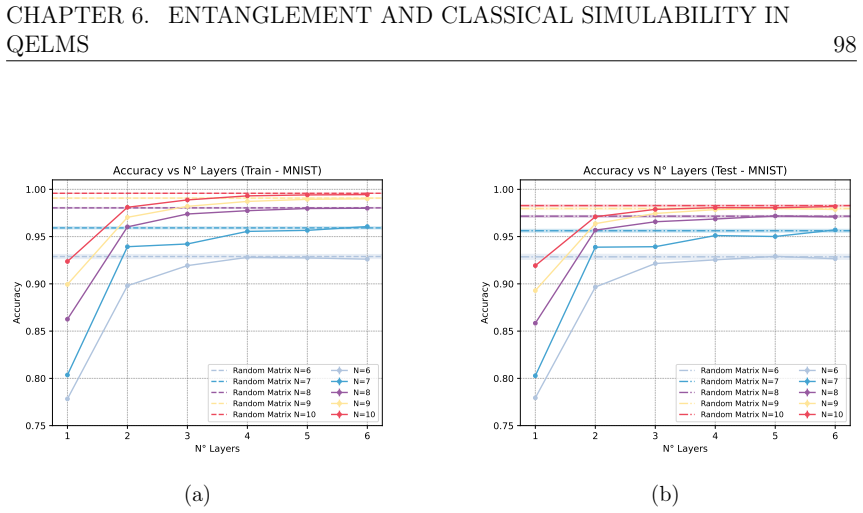
- [Sec. 6.3.2, Figs. 6.1–6.3] The equality of the XX plateau with Haar-random unitary processing is interpreted as showing that the specific structure of the XX Hamiltonian is irrelevant once the plateau is reached. An alternative explanation is that the plateau is a readout-capacity bound: for the fixed dense-angle encoded states and a linear readout on the 2^N probability simplex, any sufficiently mixing unitary could yield the same limiting accuracy A*(N). The paper does not include a classical random-feature baseline with the same 2^N-dimensional feature space (e.g., random Fourier features, a fixed random neural net, or a random linear map applied to the latent vector). Adding such a baseline would separate quantum-dynamics saturation from generic high-dimensional feature saturation.
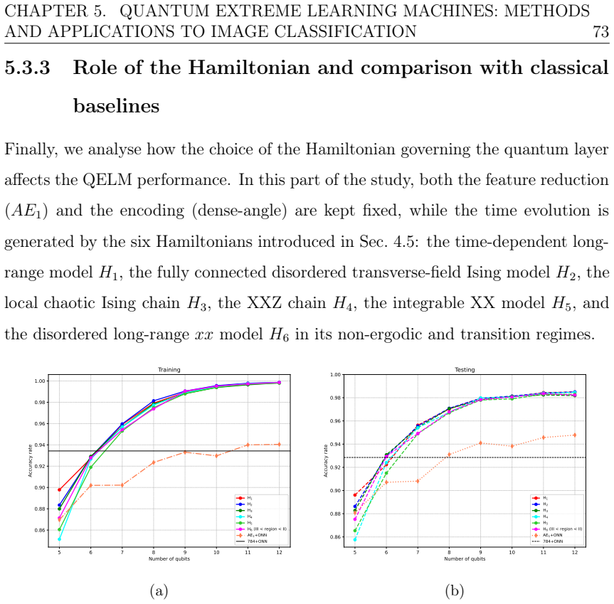
- [Sec. 5.3.3, Fig. 5.8] The first QELM study claims that the interacting quantum reservoir 'systematically improves' accuracy over classical processing, but the only classical comparisons are one-layer neural networks on raw pixels (784+ONN) or on the 2N-dimensional autoencoder latents (AE1+ONN). These baselines do not have the nonlinear capacity or feature dimensionality of the 2^N-dimensional probability readout, so they are not representative classical image classifiers. A fair comparison would use a classical nonlinear feature map of comparable dimensionality, such as random kitchen sinks, kernel ridge regression, or a CNN on the same latent inputs. This does not affect the negative quantum-advantage conclusion of Chapter 6, but it weakens the positive 'quantum reservoir enriches representation' conclusion of Chapter 5.
minor comments (6)
- [Table 4.1] The amplitude-encoding row lists '2N' features per qubit; amplitude encoding embeds 2^N features in N qubits, so the entry should be 2^N (or '2^N/N' per qubit).
- [Sec. 2.7.4] A verbatim excerpt from Ref. [50] ('are comparably good or better than the constructed solution...') appears unquoted after Eq. (2.21). If intentional, add quotation marks and a citation; if it is a formatting artifact, remove it.
- [Figs. 6.1–6.3] The legends use 'Random Matrix' while the text says 'Haar-random unitary'; please unify the terminology.
- [Sec. 4.3.2 and figure captions] Typographical issues: 'powerfullinear' missing a space in Sec. 4.3.2, and several captions read 'T esting' instead of 'Testing'.
- [Eq. (6.5)] The scaling law is written as S_N(t) ≃ N f(t/N), but the preceding notation is S_{N/2}(t) for the half-chain entropy. Define S_N explicitly or write the equation in terms of the half-chain entropy to avoid confusion.
- [General] The manuscript contains no statement about code or data availability. For a computational thesis with many numerical experiments, a repository link or a data-availability statement would improve reproducibility.
Circularity Check
No significant circularity found; central results rest on independent numerical benchmarks and analytic bounds.
full rationale
The thesis's QELM claims are supported by explicit simulations and comparisons that are not fitted to the target result: the accuracy-versus-time curves, the Haar-random unitary benchmark (Sec. 6.3.2), the one-qubit and half-chain entropy dynamics, the Lieb–Robinson velocity computed for the XX chain (Appendix A.1), and the shallow random-circuit comparison (Sec. 6.6.2) are each computed from the model or from independent baselines. The identification of the accuracy transition time t* with local entanglement is an empirical consistency argument — both the accuracy rise and the single-qubit entropy saturation occur near t ≈ 1 — rather than a reduction by construction. The paper cites the author's prior works [19,20], but those results are re-presented in the thesis with their numerical details, so the self-citations are structural, not load-bearing. No prediction is produced by renaming a fitted parameter, and no central claim is defined in terms of its own conclusion. The neutrino classification results are similarly self-contained, being benchmarked on simulated detector data with no circular dependence on the QELM analysis.
Axiom & Free-Parameter Ledger
free parameters (5)
- Evolution time (Delta t / t scan) =
Delta t=20 (H2-H6), Delta t=50T (H1); t in [1e-3, 1e2] (Ch. 6)
- Autoencoder latent dimension d =
20 (AE1/AE2 architecture dumps, Figs 5.2-5.3)
- Hamiltonian couplings and fields H1-H6 =
e.g. J0=0.06, alpha=1.51, B1=3.05 (H1); J3=-1, B3x=0.7, B3z=1.5 (H3); J4=2, J4z=0.54 (H4); B6, W in 0.02-60 (H6)
- Encoding rescaling ranges =
[0,pi] polar, [0,2pi] azimuthal (dense-angle); [0,1] populations (uniform Bloch)
- Haar-random benchmark samples =
10 unitaries per (N, dataset)
axioms (7)
- standard math Lieb-Robinson bound with vLR=1 for the nearest-neighbour XX chain
- domain assumption Computational-basis measurement is sufficiently misaligned with the XX eigenbasis to generate time-dependent, expressive features
- domain assumption Reconstruction-trained autoencoder latent space preserves class-discriminative information
- domain assumption Simulated IWCD detector images (event generation plus detector simulation, Sec. 8.3) faithfully represent real detector response
- domain assumption Haar-random unitaries are the appropriate maximal-genericity benchmark for the encoding/readout pipeline
- standard math Constant-depth Trotterized local evolution implies efficient tensor-network simulability at the relevant accuracy
- standard math Born rule / state-vector formalism of quantum mechanics
read the original abstract
This thesis investigates the application of machine-learning methods in the context of quantum computing and neutrino physics, with particular emphasis on the construction of effective representations for complex, high-dimensional data. The first part of the work is devoted to Quantum Extreme Learning Machines (QELMs), a hybrid quantum--classical framework in which classical data are encoded into quantum states and processed through fixed quantum dynamics, while learning is performed by a classical readout layer. Within this framework, we analyze the role of encoding strategies, feature-reduction methods, Hamiltonian structure, and measurement, with particular focus on the relationship between quantum dynamics, expressivity, entanglement, and classical simulability. The second part of the thesis concerns the application of deep learning to the analysis of images produced by water Cherenkov detectors in neutrino physics. Convolutional architectures, including residual networks, are developed for the classification of complex events in realistic simulated datasets, showing that such models can effectively extract relevant information from detector data. Taken together, these results highlight the potential of machine learning, in both its classical and quantum forms, as a powerful framework for the analysis of complex data in fundamental physics, while also outlining relevant challenges and directions for future research.
Figures








Reference graph
Works this paper leans on
-
[1]
Bishop.Pattern Recognition and Machine Learning
Christopher M. Bishop.Pattern Recognition and Machine Learning. Springer, New York, 2006
2006
-
[2]
MIT Press, Cambridge, MA, 2016
Ian Goodfellow, Yoshua Bengio, and Aaron Courville.Deep Learning. MIT Press, Cambridge, MA, 2016
2016
-
[3]
O’Reilly Media, 3 edition, 2022
Aurélien Géron.Hands-On Machine Learning with Scikit-Learn, Keras, and TensorFlow. O’Reilly Media, 3 edition, 2022
2022
-
[4]
Richard P. Feynman. Simulating physics with computers.Int. J. Theor. Phys., 21:467–488, 1982
1982
-
[5]
Nielsen and Isaac L
Michael A. Nielsen and Isaac L. Chuang.Quantum Computation and Quan- tum Information: 10th Anniversary Edition. Cambridge University Press, Cambridge, 2010
2010
-
[6]
Quantum algorithms: an overview.npj Quantum Inf., 2:15023, 2016
Ashley Montanaro. Quantum algorithms: an overview.npj Quantum Inf., 2:15023, 2016
2016
-
[7]
Quantum computing in the NISQ era and beyond.Quantum, 2:79, 2018
John Preskill. Quantum computing in the NISQ era and beyond.Quantum, 2:79, 2018
2018
-
[8]
Bardin, Rami Barends, Rupak Biswas, Sergio Boixo, Fernando G
Frank Arute, Kunal Arya, Ryan Babbush, Dave Bacon, Joseph C. Bardin, Rami Barends, Rupak Biswas, Sergio Boixo, Fernando G. S. L. Brandao, David A. Buell, et al. Quantum supremacy using a programmable super- conducting processor.Nature, 574:505–510, 2019
2019
-
[9]
Quantum advantage in learning from experiments.Science, 376:1182–1186, 2022
Hsin-Yuan Huang, Michael Broughton, Jordan Cotler, Sitan Chen, Jerry Li, Masoud Mohseni, Hartmut Neven, Ryan Babbush, Richard Kueng, John BIBLIOGRAPHY 160 Preskill, et al. Quantum advantage in learning from experiments.Science, 376:1182–1186, 2022
2022
-
[10]
Quantum machine learning.Nature, 549:195–202, 2017
Jacob Biamonte, Peter Wittek, Nicola Pancotti, Patrick Rebentrost, Nathan Wiebe, and Seth Lloyd. Quantum machine learning.Nature, 549:195–202, 2017
2017
-
[11]
Quantum Science and Technology
Maria Schuld and Francesco Petruccione.Supervised Learning with Quantum Computers. Quantum Science and Technology. Springer, Cham, 2018
2018
-
[12]
Quantum machine learning in feature Hilbert spaces.Phys
Maria Schuld and Nathan Killoran. Quantum machine learning in feature Hilbert spaces.Phys. Rev. Lett., 122:040504, 2019
2019
-
[13]
Springer, Cham, 2 edition, 2021
Maria Schuld and Francesco Petruccione.Machine Learning with Quantum Computers. Springer, Cham, 2 edition, 2021
2021
-
[14]
Iris Cong, Soonwon Choi, and Mikhail D. Lukin. Quantum convolutional neural networks.Nat. Phys., 15:1273–1278, 2019
2019
-
[15]
Quantum capsule networks.Quantum Sci
Zidu Liu, Pei-Xin Shen, Weikang Li, Lu-Ming Duan, and Dong-Ling Deng. Quantum capsule networks.Quantum Sci. Technol., 8:015016, 2023
2023
-
[16]
Quantum algorithms for supervised and unsupervised machine learning, 2013
Seth Lloyd, Masoud Mohseni, and Patrick Rebentrost. Quantum algorithms for supervised and unsupervised machine learning, 2013. arXiv:1307.0411 [quant-ph]
Pith/arXiv arXiv 2013
-
[17]
The quest for a quantum neural network.Quantum Inf
Maria Schuld, Ilya Sinayskiy, and Francesco Petruccione. The quest for a quantum neural network.Quantum Inf. Process., 13:2567–2586, 2014
2014
-
[18]
Córcoles, Kristan Temme, Aram W
Vojtěch Havlíček, Antonio D. Córcoles, Kristan Temme, Aram W. Harrow, Abhinav Kandala, Jerry M. Chow, and Jay M. Gambetta. Supervised learning with quantum-enhanced feature spaces.Nature, 567:209–212, 2019
2019
-
[19]
Estarellas, Nicola Lo Gullo, Thorsten Lux, Francesco Plastina, Arnau Riera, and Jacopo Set- tino
Annalisa De Lorenzis, Maria Pilar Casado, Marta P. Estarellas, Nicola Lo Gullo, Thorsten Lux, Francesco Plastina, Arnau Riera, and Jacopo Set- tino. Harnessing quantum extreme learning machines for image classification. Phys. Rev. Applied, 23:044024, 2025. BIBLIOGRAPHY 161
2025
-
[20]
Entanglement and classical simulability in quantum extreme learning machines.Phys
Annalisa De Lorenzis, Maria Pilar Casado, Nicola Lo Gullo, Thorsten Lux, Francesco Plastina, and Arnau Riera. Entanglement and classical simulability in quantum extreme learning machines.Phys. Rev. Applied, 25:054052, 2026
2026
-
[21]
Estarellas, William J
Akitada Sakurai, Marta P. Estarellas, William J. Munro, and Kae Nemoto. Quantum extreme reservoir computation utilizing scale-free networks.Phys. Rev. Applied, 17:064044, 2022
2022
-
[22]
Munro, and Kae Nemoto
Aoi Hayashi, Akitada Sakurai, Shin Nishio, William J. Munro, and Kae Nemoto. Impact of the form of weighted networks on the quantum extreme reservoir computation.Phys. Rev. A, 108:042609, 2023
2023
-
[23]
Munro, and Kae Nemoto
Aoi Hayashi, Akitada Sakurai, William J. Munro, and Kae Nemoto. Effective quantum feature maps in quantum extreme reservoir computation from the XY model.Phys. Rev. A, 111:022431, 2025
2025
-
[24]
Munro, and Kae Nemoto
Akitada Sakurai, Aoi Hayashi, William J. Munro, and Kae Nemoto. Simple Hamiltonian dynamics as a powerful resource for image classification.Phys. Rev. A, 111:052432, 2025
2025
-
[25]
Experimental property reconstruction in a photonic quantum extreme learning machine.Phys
Alessia Suprano, Danilo Zia, Luca Innocenti, Salvatore Lorenzo, Valeria Ci- mini, Taira Giordani, Ivan Palmisano, Emanuele Polino, Nicolò Spagnolo, Fabio Sciarrino, et al. Experimental property reconstruction in a photonic quantum extreme learning machine.Phys. Rev. Lett., 132:160802, 2024
2024
-
[26]
Massimo Palma
Marco Vetrano, Gabriele Lo Monaco, Luca Innocenti, Salvatore Lorenzo, and G. Massimo Palma. State estimation with quantum extreme learning machines beyond the scrambling time.npj Quantum Inf., 11:20, 2025
2025
-
[27]
Massimo Palma
Luca Innocenti, Salvatore Lorenzo, Ivan Palmisano, Alessandro Ferraro, Mauro Paternostro, and G. Massimo Palma. Potential and limitations of quantum extreme learning machines.Commun. Phys., 6:118, 2023
2023
-
[28]
Khan, and Hakan E
Gerasimos Angelatos, Saeed A. Khan, and Hakan E. Türeci. Reservoir com- puting approach to quantum state measurement.Phys. Rev. X, 11:041062, 2021. BIBLIOGRAPHY 162
2021
-
[29]
Soriano, and Roberta Zambrini
Pere Mujal, Johannes Nokkala, Rodrigo Martínez-Peña, Gian Luca Giorgi, Miguel C. Soriano, and Roberta Zambrini. Analytical evidence of nonlinear- ity in qubits and continuous-variable quantum reservoir computing.J. Phys. Complex., 2:045008, 2021
2021
-
[30]
Carlo, and Florentino Borondo
Laia Domingo, Gabriel G. Carlo, and Florentino Borondo. Optimal quantum reservoir computing for the noisy intermediate-scale quantum era.Phys. Rev. E, 106:L043301, 2022
2022
-
[31]
Sori- ano, and Roberta Zambrini
Rodrigo Martínez-Peña, Gian Luca Giorgi, Johannes Nokkala, Miguel C. Sori- ano, and Roberta Zambrini. Dynamical phase transitions in quantum reservoir computing.Phys. Rev. Lett., 127:100502, 2021
2021
-
[32]
Harnessing disordered-ensemble quantum dynamics for machine learning.Phys
Keisuke Fujii and Kohei Nakajima. Harnessing disordered-ensemble quantum dynamics for machine learning.Phys. Rev. Applied, 8:024030, 2017
2017
-
[33]
Nurdin, and Naoki Yamamoto
Jiayin Chen, Hendra I. Nurdin, and Naoki Yamamoto. Temporal information processing on noisy quantum computers.Phys. Rev. Applied, 14:024065, 2020
2020
-
[34]
Extreme learning machine: theory and applications.Neurocomputing, 70:489–501, 2006
Guang-Bin Huang, Qin-Yu Zhu, and Chee-Kheong Siew. Extreme learning machine: theory and applications.Neurocomputing, 70:489–501, 2006
2006
-
[35]
Extreme learning ma- chines: a survey.Int
Guang-Bin Huang, Dian-Hui Wang, and Yuan Lan. Extreme learning ma- chines: a survey.Int. J. Mach. Learn. Cybern., 2:107–122, 2011
2011
-
[36]
A review on extreme learning machine.Multimed
Jian Wang, Siyuan Lu, Shui-Hua Wang, and Yu-Dong Zhang. A review on extreme learning machine.Multimed. Tools Appl., 81:41611–41660, 2022
2022
-
[37]
Extreme learning machine versus classical feedforward network.Neural Comput
Urszula Markowska-Kaczmar and Michał Kosturek. Extreme learning machine versus classical feedforward network.Neural Comput. Appl., 33:15121–15144, 2021
2021
-
[38]
Extreme learning machine: algorithm, theory and applications.Artif
Shifei Ding, Han Zhao, Yanan Zhang, Xinzheng Xu, and Ru Nie. Extreme learning machine: algorithm, theory and applications.Artif. Intell. Rev., 44:103–115, 2015. BIBLIOGRAPHY 163
2015
-
[39]
Trends in extreme learning machines: a review.Neural Networks, 61:32–48, 2015
Gao Huang, Guang-Bin Huang, Shiji Song, and Keyou You. Trends in extreme learning machines: a review.Neural Networks, 61:32–48, 2015
2015
-
[40]
Avariational eigenvalue solver on a photonic quantum processor.Nat
Alberto Peruzzo, Jarrod McClean, Peter Shadbolt, Man-Hong Yung, Xiao-Qi Zhou, PeterJ.Love, AlánAspuru-Guzik, andJeremyL.O’Brien. Avariational eigenvalue solver on a photonic quantum processor.Nat. Commun., 5:4213, 2014
2014
-
[41]
Aquantumapproximate optimization algorithm, 2014
EdwardFarhi, JeffreyGoldstone, andSamGutmann. Aquantumapproximate optimization algorithm, 2014. arXiv:1411.4028 [quant-ph]
Pith/arXiv arXiv 2014
-
[42]
Benjamin, Sug- uru Endo, Keisuke Fujii, Jarrod R
Marco Cerezo, Andrew Arrasmith, Ryan Babbush, Simon C. Benjamin, Sug- uru Endo, Keisuke Fujii, Jarrod R. McClean, Kosuke Mitarai, Xiao Yuan, Lukasz Cincio, et al. Variational quantum algorithms.Nat. Rev. Phys., 3:625– 644, 2021
2021
-
[43]
Yann LeCun, Corinna Cortes, and Christopher J. C. Burges. MNIST hand- written digit database. AT&T Labs [Online]. Available:http://yann.lecun. com/exdb/mnist, 2010
2010
-
[44]
Fashion-MNIST: a novel image dataset for benchmarking machine learning algorithms, 2017
Han Xiao, Kashif Rasul, and Roland Vollgraf. Fashion-MNIST: a novel image dataset for benchmarking machine learning algorithms, 2017. arXiv:1708.07747 [cs.LG]
Pith/arXiv arXiv 2017
-
[45]
Learning multiple layers of features from tiny images
Alex Krizhevsky. Learning multiple layers of features from tiny images. Tech- nical report, Department of Computer Science, University of Toronto, 2009. Available:https://www.cs.toronto.edu/~kriz/cifar.html
2009
-
[46]
Hyper-Kamiokande Collaboration, K. Abe, et al. Hyper-Kamiokande Design Report, 2018. arXiv:1805.04163 [physics.ins-det]
Pith/arXiv arXiv 2018
-
[47]
Abe, et al
Hyper-Kamiokande Collaboration, K. Abe, et al. Physics potential of a long- baseline neutrino oscillation experiment using a J-PARC neutrino beam and Hyper-Kamiokande.Prog. Theor. Exp. Phys., 2015:053C02, 2015. BIBLIOGRAPHY 164
2015
-
[48]
Abe, et al
Hyper-Kamiokande Collaboration, K. Abe, et al. Sensitivity of the Hyper- Kamiokande experiment to neutrino oscillation parameters using accelerator neutrinos.Eur. Phys. J. C, 86:170, 2026
2026
-
[49]
Abe, et al
Hyper-Kamiokande Collaboration, K. Abe, et al. The Hyper-Kamiokande experiment: input to the update of the European Strategy for Particle Physics,
-
[50]
Deep residual learning for image recognition
Kaiming He, Xiangyu Zhang, Shaoqing Ren, and Jian Sun. Deep residual learning for image recognition. InProc. IEEE Conf. Comput. Vis. Pattern Recognit., pages 770–778, 2016
2016
-
[51]
WatChMaL: Water Cherenkov machine learning
WatChMaL Collaboration. WatChMaL: Water Cherenkov machine learning. GitHub repository. Available:https://github.com/WatChMaL/WatChMaL, 2020
2020
-
[52]
Arthur L. Samuel. Some studies in machine learning using the game of check- ers.IBM J. Res. Dev., 3:210–229, 1959
1959
-
[53]
Wiley, New York, 1949
DonaldO.Hebb.The Organization of Behavior: A Neuropsychological Theory. Wiley, New York, 1949
1949
-
[54]
McCulloch and Walter Pitts
Warren S. McCulloch and Walter Pitts. A logical calculus of the ideas imma- nent in nervous activity.Bull. Math. Biophys., 5:115–133, 1943
1943
-
[55]
Rumelhart, Geoffrey E
David E. Rumelhart, Geoffrey E. Hinton, and Ronald J. Williams. Learning representations by back-propagating errors.Nature, 323:533–536, 1986
1986
-
[56]
Support-vector networks.Mach
Corinna Cortes and Vladimir Vapnik. Support-vector networks.Mach. Learn., 20:273–297, 1995
1995
-
[57]
Deep learning.Nature, 521:436–444, 2015
Yann LeCun, Yoshua Bengio, and Geoffrey Hinton. Deep learning.Nature, 521:436–444, 2015
2015
-
[58]
Maddison, Arthur Guez, Laurent Sifre, George van den Driessche, Julian Schrittwieser, Ioannis Antonoglou, Veda BIBLIOGRAPHY 165 Panneershelvam, Marc Lanctot, et al
David Silver, Aja Huang, Chris J. Maddison, Arthur Guez, Laurent Sifre, George van den Driessche, Julian Schrittwieser, Ioannis Antonoglou, Veda BIBLIOGRAPHY 165 Panneershelvam, Marc Lanctot, et al. Mastering the game of Go with deep neural networks and tree search.Nature, 529:484–489, 2016
2016
-
[59]
Pankaj Mehta, Marin Bukov, Ching-Hao Wang, Alexandre G. R. Day, Clint Richardson, CharlesK.Fisher, andDavidJ.Schwab. Ahigh-bias, low-variance introduction to machine learning for physicists.Phys. Rep., 810:1–124, 2019
2019
-
[60]
Approximation by superpositions of a sigmoidal function
George Cybenko. Approximation by superpositions of a sigmoidal function. Math. Control Signal Systems, 2:303–314, 1989
1989
-
[61]
Multilayer feed- forward networks are universal approximators.Neural Networks, 2:359–366, 1989
Kurt Hornik, Maxwell Stinchcombe, and Halbert White. Multilayer feed- forward networks are universal approximators.Neural Networks, 2:359–366, 1989
1989
-
[62]
Gradient- based learning applied to document recognition.Proc
Yann LeCun, Leon Bottou, Yoshua Bengio, and Patrick Haffner. Gradient- based learning applied to document recognition.Proc. IEEE, 86:2278–2324, 1998
1998
-
[63]
Cam- bridge University Press, Cambridge, 3 edition, 2020
Jun John Sakurai and Jim Napolitano.Modern Quantum Mechanics. Cam- bridge University Press, Cambridge, 3 edition, 2020
2020
-
[64]
echo state
Herbert Jaeger. The “echo state” approach to analysing and training recurrent neural networks. GMD Report 148, German National Research Center for Information Technology, 2001
2001
-
[65]
Real-time com- puting without stable states: a new framework for neural computation based on perturbations.Neural Comput., 14:2531–2560, 2002
Wolfgang Maass, Thomas Natschläger, and Henry Markram. Real-time com- puting without stable states: a new framework for neural computation based on perturbations.Neural Comput., 14:2531–2560, 2002
2002
-
[66]
Soriano, and Roberta Zambrini
Pere Mujal, Rodrigo Martínez-Peña, Johannes Nokkala, Jorge García-Beni, Gian Luca Giorgi, Miguel C. Soriano, and Roberta Zambrini. Opportunities in quantum reservoir computing and extreme learning machines.Adv. Quantum Technol., 4:2100027, 2021
2021
-
[67]
On fundamental aspects of quantum extreme learning machines.Quantum Mach
Weijie Xiong, Giorgio Facelli, Mehrad Sahebi, Owen Agnel, Thiparat Chotibut, Supanut Thanasilp, and Zoë Holmes. On fundamental aspects of quantum extreme learning machines.Quantum Mach. Intell., 7:20, 2025. BIBLIOGRAPHY 166
2025
-
[68]
Marco Cerezo, Guillaume Verdon, Hsin-Yuan Huang, Lukasz Cincio, and Patrick J. Coles. Challenges and opportunities in quantum machine learn- ing.Nat. Comput. Sci., 2:567–576, 2022
2022
-
[69]
Fiderer, Hendrik Poulsen Nautrup, Jonas M
Sofiene Jerbi, Lukas J. Fiderer, Hendrik Poulsen Nautrup, Jonas M. Kübler, Hans J. Briegel, and Vedran Dunjko. Quantum machine learning beyond kernel methods.Nat. Commun., 14:517, 2023
2023
-
[70]
Hsin-Yuan Huang, Michael Broughton, Masoud Mohseni, Ryan Babbush, Ser- gio Boixo, Hartmut Neven, and Jarrod R. McClean. Power of data in quantum machine learning.Nat. Commun., 12:2631, 2021
2021
-
[71]
McClean, Sergio Boixo, Vadim N
Jarrod R. McClean, Sergio Boixo, Vadim N. Smelyanskiy, Ryan Babbush, and Hartmut Neven. Barren plateaus in quantum neural network training landscapes.Nat. Commun., 9:4812, 2018
2018
-
[72]
Samson Wang, Enrico Fontana, Marco Cerezo, Kunal Sharma, Akira Sone, Lukasz Cincio, and Patrick J. Coles. Noise-induced barren plateaus in varia- tional quantum algorithms.Nat. Commun., 12:6961, 2021
2021
-
[73]
Soriano, and Roberta Zambrini
Jorge García-Beni, Iris Paparelle, Valentina Parigi, Gian Luca Giorgi, Miguel C. Soriano, and Roberta Zambrini. Quantum machine learning via continuous-variable cluster states and teleportation.EPJ Quant. Technol., 12:63, 2025
2025
-
[74]
Nicoli, Paolo Stornati, Rouven Koch, Miriam Büttner, et al.Machine learning in quantum sciences
Anna Dawid, Julian Arnold, Borja Requena, Alexander Gresch, Marcin Płodzień, Kaelan Donatella, Kim A. Nicoli, Paolo Stornati, Rouven Koch, Miriam Büttner, et al.Machine learning in quantum sciences. Cambridge University Press, 2025
2025
-
[75]
La- torre
Adrián Pérez-Salinas, Alba Cervera-Lierta, Elies Gil-Fuster, and José I. La- torre. Data re-uploading for a universal quantum classifier.Quantum, 4:226, 2020. BIBLIOGRAPHY 167
2020
-
[76]
Harnessing quantum backaction for time-series processing
Giacomo Franceschetto, Marcin Płodzień, Maciej Lewenstein, Antonio Acín, and Pere Mujal. Harnessing quantum backaction for time-series processing. Phys. Rev. X, 16:021002, 2026
2026
-
[77]
An insight into extreme learning machines: random neu- rons, random features and kernels.Cogn
Guang-Bin Huang. An insight into extreme learning machines: random neu- rons, random features and kernels.Cogn. Comput., 6:376–390, 2014
2014
-
[78]
Extreme learning machine: a new learning scheme of feedforward neural networks
Guang-Bin Huang, Qin-Yu Zhu, and Chee Kheong Siew. Extreme learning machine: a new learning scheme of feedforward neural networks. InProc. IEEE Int. Joint Conf. Neural Networks, volume 2, pages 985–990, 2004
2004
-
[79]
Solanki and Anh Pham
Payal D. Solanki and Anh Pham. Harnessing quantum dynamics for robust and scalable quantum extreme learning machines.Phys. Rev. A, 113:042443, 2026
2026
-
[80]
Entanglement estimation of Werner states with a quantum extreme learning machine.Phys
Hajar Assil, Abderrahim El Allati, and Gian Luca Giorgi. Entanglement estimation of Werner states with a quantum extreme learning machine.Phys. Rev. A, 111:022412, 2025
2025
discussion (0)
Sign in with ORCID, Apple, or X to comment. Anyone can read and Pith papers without signing in.