REVIEW 3 major objections 5 minor 44 references
Beyond Constant Error: Heteroscedastic Bayesian Model Combination for Modeling Unmeasured Nuclei
T0 review · 3 major / 5 minor · reviewed 2026-08-02 · deepseek-v4-flash
Pith's one-line read A Bayesian ensemble method with error bars that grow with model disagreement and extrapolation distance calibrates nuclear uncertainties more honestly than constant-variance error bars, especially near the drip lines.
desk verdict Useful heteroscedastic extension of BMC with solid synthetic validation, but the key distance predictor is undefined and validation is used for selection—fixable before acceptance. read the letter →
The pith
A machine-rendered reading of the paper's core claim, the machinery that carries it, and where it could break.
The reading
What carries the argument
The central object is the heteroscedastic error scale σ_i² = α + β₁ d_i + γ₁ v_i, built from two predictors: d_i, a distance in the principal-component space of the model ensemble, and v_i, the variance of individual model predictions at each nucleus. This scale replaces the single global σ₀ of the homoscedastic model, letting the likelihood and posterior allocate more uncertainty to nuclei where models extrapolate far from the data or disagree strongly. The BMC weights are still calibrated on principal components of the centered model matrix, but now every posterior sample carries its own error scale, so reported credible intervals reflect both weight uncertainty and error-model uncertainty
What would settle it
Recompute the heteroscedastic model with d_i defined as the Euclidean distance from the training-data centroid in principal-component space (or in the original (N,Z) grid) and compare calibration metrics; if the improvement over homoscedastic error disappears or inverts, the current d_i is not measuring extrapolation distance and the physical motivation for the growing error bands collapses.
Extended reading notes
Core claim
The paper establishes that a heteroscedastic error model, with variance σ_i² = α + β₁ d_i + γ₁ v_i where d_i is a distance in principal-component space and v_i is the inter-model variance, outperforms a constant-variance homoscedastic error model for calibrating uncertainty in extrapolated separation energies. On six synthetic benchmarks, the heteroscedastic model brings the average reduced chi-squared from 1.32 down to about 1.08, and on real data it consistently lowers the MACE relative to the homoscedastic baseline. The resulting drip-line existence probabilities inherit the growing uncertainty, producing smoother transitions from bound to unbound regions rather than artificially sharp cu
Load-bearing premise
The load-bearing premise is that d_i genuinely measures how far a nucleus is from the training data in principal-component space, but the paper never explicitly defines d_i; if d_i does not track extrapolation distance, the claimed calibration improvement may be an artifact of the predictor choice rather than a physical effect.
Editorial extensions
If this is right
- Drip-line existence probabilities become more conservative and graded: nuclei in regions of strong model disagreement receive non-trivial existence probabilities even when the central prediction is negative.
- Validation-set calibration metrics (MACE) become a reliable proxy for deep-extrapolation performance, allowing practitioners to select error models without direct access to unknown territory.
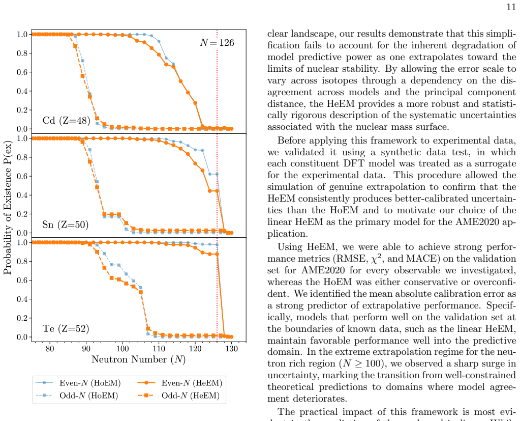
- The method distinguishes regions where extrapolation is genuinely unconstrained from regions where models agree despite distance, such as the N=126 shell gap, where uncertainty growth is moderated.
- New mass measurements near the limits of stability, such as the recent Cd and Te data, provide direct tests of whether the heteroscedastic bands are honestly sized; the paper shows such comparisons for ⁹⁶⁻⁹⁸Cd and ¹⁰⁴Te.
Reading between the lines
- The paper never explicitly defines d_i — it is introduced as a 'distance from the center of the training data in PC space,' but the PC-space origin is the ensemble-mean model. Recomputing results with d_i defined as a genuine Euclidean distance to the training-data centroid would test whether the claimed calibration gains are driven by true extrapolation distance or by the variance term alone.
- Because the homoscedastic model is nested within the heteroscedastic one, a posterior comparison of α, β₁, γ₁ could yield a formal Bayes factor for whether heteroscedasticity is statistically required for a given observable, extending beyond the paper's metric-based argument.
- The same variance-function approach should transfer to any ensemble of physical models with two available diagnostics — an extrapolation distance and an inter-model spread — such as climate or materials-science ensembles, where constant-error assumptions are equally common and equally suspect.
- A natural next step would be to use the heteroscedastic error model's Q_alpha predictions as calibration data to refit energy density functionals in the ¹⁰⁰Sn region, a direction the paper hints at but does not pursue.
Editorial analysis
A structured set of objections, weighed in public.
Referee Report
Summary. The manuscript introduces a heteroscedastic extension of Bayesian Model Combination (BMC) for nuclear mass predictions. In place of a constant error scale (HoEM), the error variance is modeled as σ_i^2 = α + β_1 d_i + γ_1 v_i, where d_i is described as a distance in principal-component space and v_i is the variance among the six EDF predictions (Eq. 13b). The parameters are inferred jointly with the BMC weights on AME2020 training data. The paper validates the method with leave-one-model-out synthetic experiments (Tables I–II) and with held-out validation data for Z = 46–52 (Tables III–V), reporting improved reduced χ² and MACE for the linear HeEM. It then applies HeEM to separation energies, Q_α, and drip-line existence probabilities.
Significance. The proposal is timely: the constant-variance assumption is a recognized limitation in multi-model nuclear UQ, and the heteroscedastic form is simple and physically motivated. The synthetic validation is a genuine strength: six independent leave-one-out experiments with different surrogate models provide evidence that the calibration gain is not an artifact of one benchmark. The real-data validation against AME2020 and the two new experimental comparisons (Cd masses, 104Te Q_α) are also valuable. If the ambiguities around the distance predictor and validation protocol are resolved, the paper would make a solid contribution to uncertainty quantification in nuclear theory.
major comments (3)
- [§III.A, Eqs. (12)–(13b)] The key predictor d_i is never defined. The text calls it 'distance from the center of the training data in PC space,' but Eq. (12) defines coordinates ζ_i by projecting the centered deviation vector x_c^i = x_0^i − φ_0(x_i) onto the SVD axes. The origin of this PC space is the ensemble-mean model, not the centroid of the training-set projections. A nucleus far from known data with model consensus can have small ||ζ_i||, so d_i as written need not measure extrapolation distance. Since d_i is the first driver in Eq. (13b), the physical rationale for the expanding HeEM bands is not established. Please define d_i explicitly (e.g., distance from the training-data centroid in PC space), report its empirical correlation with validation residuals, and state whether the reported results are robust to that definition.
- [§III (p selection) and §IV–V (validation)] The validation set is used both to select hyperparameters (the number of retained components p) and to choose between linear and quadratic HeEM, and the same set is then used to report the headline calibration metrics in Tables I–V. This double use can bias the reported improvements. Please either split off a separate test set, perform nested cross-validation, or at minimum quantify how much of the HeEM advantage survives when p and model form are fixed a priori.
- [Table II and §IV] The claim that validation-set MACE is a strong predictor of extrapolation performance is supported by the synthetic experiment, but the comparison between validation and prediction-set MACE is presented without uncertainty estimates. Given that only six surrogate models are used, the average improvements (e.g., validation MACE 7.31 vs. 10.90) could be sensitive to one or two leave-one-out folds. Reporting per-fold MACE or a standard error would strengthen this inference.
minor comments (5)
- [Eq. (15)] The text says M is 'the number of samples in the validation or test dataset,' but MACE is averaged over credible interval levels. M should be the number of p_j values used in the calibration curve.
- [Table II caption] The caption says 'MACE score averaged across error models,' but the table appears to average across synthetic surrogate models, not error models. Please clarify.
- [Table V caption] The caption reads 'proton and separation energies'; this should be 'proton and neutron separation energies.'
- [Fig. 2] The figure caption refers to 'distance (11),' but Eq. (11) defines Δ(N,Z). Please clarify whether the plotted quantity is exactly Δ(N,Z) or a scaled version.
- [§III.A] The posterior values of the error-model parameters α, β_1, γ_1 are not reported. Reporting their posterior means and credible intervals would help readers judge whether the inferred distance and variance dependencies are physically reasonable.
Circularity Check
No significant circularity: HeEM calibration gains are supported by held-out validation and synthetic leave-one-model-out tests.
full rationale
The paper's central claim—that the heteroscedastic error scale of Eq. (13b), sigma_i^2 = alpha + beta_1 d_i + gamma_1 v_i, yields better-calibrated uncertainty than the homoscedastic Eq. (13a)—is not circular. The parameters (alpha, beta_1, gamma_1) are sampled from the posterior (Eq. 10) using training-set data, while the evidence for superior calibration is produced on two independent holdouts: the AME2020 validation set (outermost measured nuclei, 30/70 split) and a synthetic leave-one-model-out experiment where each DFT model is excluded in turn and used as the surrogate truth. The error-model predictors d_i and v_i are constructed from the model ensemble and the PC decomposition (Eqs. 3-6, 12), not from the target residuals or from the reported MACE/chi^2 metrics, so Eq. (13b) does not reduce to the quantity it is claimed to predict. The BMC basis and weight priors follow Ref. [13] by the same group, and Ref. [14] is a prior application; these self-citations supply the baseline framework but are shared by HoEM and HeEM and do not force the HeEM result. The paper even reports a case where the HeEM error model fails (97Cd, where a common model bias is not captured by v_i), demonstrating that the framework is falsifiable rather than true by construction. The reader-identified ambiguity in d_i—the PC-space origin is the ensemble-mean model rather than an explicitly defined training-data centroid—is a specification/correctness concern, not a circular identity: it affects whether the error model is physically well motivated, but the calibration comparison remains an empirical, held-out comparison. Score 2 reflects only the presence of minor, non-load-bearing self-citations; no circular step was identified.
Assumptions & free parameters
free parameters (5)
- BMC weights b_j =
not reported (posterior means)
- Error-model intercept alpha =
not reported
- HeEM linear coefficients beta_1, gamma_1 =
not reported
- Number of retained principal components p =
not reported
- Prior widths for b from SVD =
not reported
assumptions (7)
- standard math SVD/PCA decomposition and truncation of the centered model matrix (Eq. 5) yields a valid reduced basis for the BMC.
- domain assumption Residuals are conditionally independent with likelihood p(y|b,Lambda) as in Eq. (9).
- domain assumption Positivity of sigma_i^2 is enforced by positive priors and rejection of violating proposals (Sec. III A).
- ad hoc to paper The predictors d_i (PC-space distance) and v_i (model variance) are sufficient and correctly specified for the theoretical error.
- domain assumption Validation-set calibration performance is a reliable proxy for deep-extrapolation performance.
- domain assumption The six EDFs satisfy the 'reasonable model' criterion and are diverse enough that inter-model variance v_i encodes missing physics.
- domain assumption The nuclear DFT calculations assume axial deformation, reflection invariance, and equal-filling approximation for odd-A and odd-odd nuclei.
Cite this review
Pith. "Pith review of Beyond Constant Error: Heteroscedastic Bayesian Model Combination for Modeling Unmeasured Nuclei." pith.science (2026). https://pith.science/paper/VGLWYXH4
@misc{pith2026260714039,
  author       = {Pith},
  title        = {Pith review of: Beyond Constant Error: Heteroscedastic Bayesian Model Combination for Modeling Unmeasured Nuclei},
  year         = {2026},
  howpublished = {\url{https://pith.science/paper/VGLWYXH4}},
  note         = {Machine review of arXiv:2607.14039}
}
abstract
Experimentally inaccessible regions of the nuclear chart remain a challenge for global models of atomic nuclei to predict. This includes exotic nuclei near particle drip lines, superheavy elements at the extremes of mass and charge, and the neutron-rich pathways of astrophysical processes in explosive stellar environments where heavy elements are created. Given that individual nuclear models are imperfect, deep extrapolations are best approached using model ensembles, which allow for the systematic combination of diverse theoretical predictions. In this study, we employ the recently introduced Bayesian Model Combination (BMC) method, based on statistical machine learning, that provides robust uncertainty quantification for forecasts using model ensembles. To account for the inherent degradation of predictive power as models extrapolate into the yet-unexplored domain, we introduce a heteroscedastic BMC framework in which the combined theoretical uncertainty is treated as a dynamic quantity. We apply this methodology to an ensemble of realistic energy density functionals with a specific focus on the $Z=46\text{--}52$ isotopic chains. We rigorously validate the approach using both experimental data and synthetic data designed to assess performance in the deep extrapolation regime. Our results demonstrate that the proposed heteroscedastic approach yields superior calibration metrics and provides statistically principled assessments of the particle drip lines.
Figures


Figures from the paper (6 more)


Reference graph
Works this paper leans on
-
[1]
(10), are ob- tained by using a Gibbs sampler
In all cases, samples from the posterior, Eq. (10), are ob- tained by using a Gibbs sampler. For the homoscedastic model this is a standard two-block Gibbs sampler, while the heteroscedastic model uses Metropolis–Hastings step embedded within each Gibbs sweep (a Metropolis-within- Gibbs scheme) [34]. The point predictions reported in our validation tables...
2018
-
[2]
Neufcourt, Y
L. Neufcourt, Y. Cao, S. A. Giuliani, W. Nazarewicz, E. Olsen, and O. B. Tarasov, Quantified limits of the nuclear landscape, Phys. Rev. C101, 044307 (2020)
2020
-
[3]
Erler, N
J. Erler, N. Birge, M. Kortelainen, W. Nazarewicz, E. Olsen, A. M. Perhac, and M. Stoitsov, The limits of the nuclear landscape, Nature486, 509 (2012)
2012
-
[4]
J. J. Cowan, C. Sneden, J. E. Lawler, A. Aprahamian, M. Wiescher, K. Langanke, G. Mart ´ ınez-Pinedo, and F.- K. Thielemann, Origin of the heaviest elements: The rapid neutron-capture process, Rev. Mod. Phys.93, 015002 (2021)
2021
-
[5]
S. R. Stroberg, J. D. Holt, A. Schwenk, and J. Simonis, Ab initio limits of atomic nuclei, Phys. Rev. Lett.126, 022501 (2021)
2021
-
[6]
Schunck, ed.,Energy Density Functional Methods for Atomic Nuclei, 2053-2563 (IOP Publishing, 2019)
N. Schunck, ed.,Energy Density Functional Methods for Atomic Nuclei, 2053-2563 (IOP Publishing, 2019)
-
[7]
Bender, P.-H
M. Bender, P.-H. Heenen, and P.-G. Reinhard, Self- consistent mean-field models for nuclear structure, Rev. Mod. Phys.75, 121 (2003)
2003
-
[8]
Q. Yuan, P. Qi, X. Xiao, X. Wang, J. He, G. Long, Z. Duan, Y. Dai, R. Yan, G. Yu, and H. Yang, Machine learning-driven high-precision model forα-decay en- ergy and half-life prediction of superheavy nuclei, Phys. Scripta101, 176004 (2026), arXiv:2508.03155 [nucl-th]
arXiv 2026
Show all 44 references
-
[9]
Schunck, J
N. Schunck, J. D. McDonnell, J. Sarich, S. M. Wild, and D. Higdon, Error analysis in nuclear density functional theory, J. Phys. G: Nucl. Part. Phys.42, 034024 (2015)
2015
-
[10]
Neufcourt, Y
L. Neufcourt, Y. Cao, W. Nazarewicz, and F. Viens, Bayesian approach to model-based extrapolation of nu- clear observables, Phys. Rev. C98, 034318 (2018)
2018
-
[11]
Utama, J
R. Utama, J. Piekarewicz, and H. B. Prosper, Nuclear mass predictions for the crustal composition of neutron stars: A bayesian neural network approach, Phys. Rev. C93, 014311 (2016)
2016
-
[12]
Neufcourt, Y
L. Neufcourt, Y. Cao, W. Nazarewicz, E. Olsen, and F. Viens, Neutron drip line in the Ca region from Bayesian model averaging, Phys. Rev. Lett.122, 062502 (2019)
2019
-
[13]
Kejzlar, L
V. Kejzlar, L. Neufcourt, and W. Nazarewicz, Local Bayesian Dirichlet mixing of imperfect models, Sci. Rep. 13, 19600 (2023)
2023
-
[14]
C. M. Ireland, G. Bollen, S. E. Campbell, X. Chen, H. Erington, N. D. Gamage, K. Godbey, A. M. Houff, C. Izzo, B. Knight, S. Lalit, E. Leistenschneider, E. M. Lykiardopoulou, F. M. Maier, W. Nazarewicz, R. Orford, W. S. Porter, C. Quick, A. Ravli´ c, M. Redshaw, P.-G. Reinhard...
2026
-
[15]
Giuliani, K
P. Giuliani, K. Godbey, V. Kejzlar, and W. Nazarewicz, Model orthogonalization and Bayesian forecast mixing via principal component analysis, Phys. Rev. Res.6, 033266 (2024)
2024
-
[16]
Y¨ uksel, T
E. Y¨ uksel, T. Marketin, and N. Paar, Optimizing the relativistic energy density functional with nuclear ground state and collective excitation properties, Phys. Rev. C 99, 034318 (2019)
2019
-
[17]
Nikˇ si´ c, D
T. Nikˇ si´ c, D. Vretenar, and P. Ring, Relativistic nu- clear energy density functionals: Adjusting parameters to binding energies, Phys. Rev. C78, 034318 (2008)
2008
-
[18]
Kortelainen, J
M. Kortelainen, J. McDonnell, W. Nazarewicz, P.-G. Reinhard, J. Sarich, N. Schunck, M. V. Stoitsov, and S. M. Wild, Nuclear energy density optimization: Large deformations, Phys. Rev. C85, 024304 (2012)
2012
-
[19]
G. A. Lalazissis, T. Nikˇ si´ c, D. Vretenar, and P. Ring, New relativistic mean-field interaction with density- dependent meson-nucleon couplings, Phys. Rev. C71, 024312 (2005)
2005
-
[20]
Karthein, C
J. Karthein, C. M. Ricketts, R. F. G. Ruiz,et al., Elec- tromagnetic properties of indium isotopes elucidate the doubly magic character of 100Sn, Nat. Phys.20, 1719 (2024)
2024
-
[21]
Kortelainen, J
M. Kortelainen, J. McDonnell, W. Nazarewicz, E. Olsen, P.-G. Reinhard, J. Sarich, N. Schunck, S. M. Wild, D. Davesne, J. Erler, and A. Pastore, Nuclear energy density optimization: Shell structure, Phys. Rev. C89, 054314 (2014)
2014
-
[22]
Reinhard and W
P.-G. Reinhard and W. Nazarewicz, Toward a global de- scription of nuclear charge radii: Exploring the Fayans energy density functional, Phys. Rev. C95, 064328 (2017)
2017
-
[23]
Tian, Z.-y
Y. Tian, Z.-y. Ma, and P. Ring, Axially deformed rela- tivistic Hartree Bogoliubov theory with a separable pair- ing force, Phys. Rev. C80, 024313 (2009)
2009
-
[24]
Marevi´ c, N
P. Marevi´ c, N. Schunck, E. Ney, R. Navarro P´ erez, M. Verriere, and J. O’Neal, Axially-deformed solution of the Skyrme-Hartree-Fock-Bogoliubov equations using the transformed harmonic oscillator basis (IV) hfbtho (v4.0): A new version of the program, Comput. Phys. Commun.27...
2022
-
[25]
Nikˇ si´ c, N
T. Nikˇ si´ c, N. Paar, D. Vretenar, and P. Ring, DIRHB—A relativistic self-consistent mean-field frame- work for atomic nuclei, Comput. Phys. Commun.185, 1808 (2014)
2014
-
[26]
Perez-Martin and L
S. Perez-Martin and L. M. Robledo, Microscopic justifi- cation of the equal filling approximation, Phys. Rev. C 78, 014304 (2008)
2008
-
[27]
Reinhard, B
P.-G. Reinhard, B. Schuetrumpf, and J. Maruhn, The Axial Hartree–Fock + BCS Code SkyAx, Comput. Phys. Commun.258, 107603 (2021)
2021
-
[28]
A. Blum, J. Hopcroft, and R. Kannan,Foundations of Data Science(Cambridge University Press, 2020)
2020
-
[29]
M. Wang, W. Huang, F. Kondev, G. Audi, and S. Naimi, The AME2020 atomic mass evaluation (II). Tables, graphs and references, Chin. Phys. C45, 030003 (2021)
2021
-
[30]
S. L. Brunton and J. N. Kutz,Data-driven science and engineering: Machine learning, dynamical systems, and control(Cambridge University Press, 2019)
2019
-
[31]
Jolliffe,Principal Component Analysis, Springer Series in Statistics (Springer, 2002)
I. Jolliffe,Principal Component Analysis, Springer Series in Statistics (Springer, 2002)
2002
-
[32]
R. J. Carroll and D. Ruppert,Transformation and weighting in regression(Chapman and Hall/CRC, 2017)
2017
-
[33]
Gelman, J
A. Gelman, J. B. Carlin, H. S. Stern, and D. B. Rubin, Bayesian data analysis, 3rd ed., Texts in Statistical Sci- ence Series (Chapman & Hall/CRC, Boca Raton, FL,
-
[34]
P. D. Hoff,A first course in Bayesian statistical methods, Vol. 580 (Springer, 2009). 13
2009
-
[35]
Davidian and R
M. Davidian and R. J. Carroll, Variance function estima- tion, Journal of the American statistical association82, 1079 (1987)
1987
-
[36]
T. P. Morris, I. R. White, and M. J. Crowther, Using sim- ulation studies to evaluate statistical methods, Statistics in Medicine38, 2074 (2019)
-
[37]
Schall, The empirical coverage of confidence intervals: Point estimates and confidence intervals for confidence levels, Biometrical Journal54, 537 (2012)
R. Schall, The empirical coverage of confidence intervals: Point estimates and confidence intervals for confidence levels, Biometrical Journal54, 537 (2012)
2012
-
[38]
Gneiting, F
T. Gneiting, F. Balabdaoui, and A. E. Raftery, Proba- bilistic forecasts, calibration and sharpness, J. Roy. Stat. Soc. Ser. B Stat. Methodol.69, 243 (2007)
2007
-
[39]
Kuleshov, N
V. Kuleshov, N. Fenner, and S. Ermon, Accurate un- certainties for deep learning using calibrated regression, inProceedings of the 35th International Conference on Machine Learning, Proceedings of Machine Learning Re- search, Vol. 80, edited by J. Dy and A. Krause (PMLR,
-
[40]
Lange, D
D. Lange, D. Atanasov, M. Au, A. Belley, M. Ben- hatchi, K. Blaum, R. B. Cakirli, P. F. Giesel, A. Her- lert, J. D. Holt, B. S. Hu, A. Jaries, C. Klink, Y. A. Litvinov, D. Lunney, V. Manea, F. Mehlhorn, T. Miyagi, M. Mougeot, S. Naimi, L. Nies, M. Schlaich, C. Schweiger, L. Sc...
2026 arXiv
-
[41]
underestimate the true deviation
and recent [42] experimental values. underestimate the true deviation. TABLE VI. Predictions and newly established experimental values (in MeV) forS 1n in 96−98Cd. The experimental values are derived from the mass excesses reported in Ref. [40], uti- lizing the extrapolated ma...
-
[42]
Gneiting and A
T. Gneiting and A. E. Raftery, Strictly proper scoring rules, prediction, and estimation, J. Amer. Statist. Assoc. 102, 359 (2007)
2007
-
[43]
Auranen, D
K. Auranen, D. Seweryniak, M. Albers, A. D. Ayangeakaa, S. Bottoni, M. P. Carpenter, C. J. Chiara, P. Copp, H. M. David, D. T. Doherty, J. Harker, and C. R. Hoffman, Superallowedαdecay to doubly magic 100Sn, Phys. Rev. Lett.121, 182501 (2018)
2018
-
[44]
I. Cox, R. Grzywacz, T. T. King, K. P. Rykaczewski, S. Nishimura, R. Yokoyama, N. Fukuda, N. Kitamura, S. Go, C. Mazzocchi, J. M. Allmond, A. Augustyn, N. Braukman, P. Brionnet, A. Esmaylzadeh, J. Fis- cher, G. Garcia de Lorenzo, S. Hanai, D. Hoskins, N. Imai, K. Kolos, A. Kor...
2026
Reviewed August 2, 2026 · model on record in the stance chip above.
Discussion (0). Continue with ORCID to comment.