REVIEW 3 major objections 6 minor 47 references
Generalized Neural Distributional Regression
T0 review · 3 major / 6 minor · reviewed 2026-08-02 · deepseek-v4-flash
Pith's one-line read By freezing a deep network's hidden layers as a fixed basis expansion, the terminal layer becomes a classical MLE with recoverable Fisher information — observation-specific confidence bands follow for any distributional parameter.
desk verdict A genuinely useful two-step MLE framework with a real conditional-inference caveat: the reported intervals ignore first-step feature-estimator uncertainty, and the test-set model selection weakens the empirical claims. read the letter →
The pith
A machine-rendered reading of the paper's core claim, the machinery that carries it, and where it could break.
The reading
What carries the argument
The load-bearing device is the two-step estimation split ω = {ω_deep, ω_last}. Step 1 optimizes the full network by stochastic gradient methods; step 2 permanently freezes ω̂_deep, so the final hidden layer becomes a deterministic learned basis expansion v(x) = F_deep(x; ω̂_deep), and the network output collapses to the linear form F(x; ω) = W_lastᵀ v(x) + b_last. With the structured effects ξ, the model is then exactly a vector generalized linear model — a linear model for several distribution parameters at once — over the identifiable parameter vector θ_last = (ξ, vec(W_last), b_last), whose design matrix [z, v(x)] is full rank thanks to the disjoint-covariate condition. The observed Fishe
What would settle it
Simulate data from a GNDR model whose true parameters are known, with a wide terminal bottleneck so the learned features carry nontrivial estimation error. Fit the two-step procedure across many Monte Carlo replicates and compare the empirical standard deviation of θ̂_last with the mean inverse observed Hessian: if the ratio deviates from one, or if Delta-method interval coverage falls below nominal while a full two-step bootstrap holds nominal coverage, then Theorem 1's conditional characterization is incomplete.
Extended reading notes
Core claim
Conditional on the frozen latent feature vectors v(x_i) produced by the upstream network, the GNDR estimator θ̂_last is asymptotically normal: √n(θ̂_last − θ_last⁰) → N_q(0, Σ_last) with Σ_last = I⁻¹(θ_last⁰) (Theorem 1). Because the second training step drives the restricted log-likelihood to a strict root of the score equation over a fixed, finite-dimensional parameter space, standard regularity conditions for vector generalized linear models apply, and the inverse observed Hessian (Eq. 8) is a machine-precision-accurate covariance estimate. From this anchor, the paper chains three Delta-method applications — through the data-dependent projection P(x), the predictor mapping h, and the inve
Load-bearing premise
The entire inferential output treats the deep features from the first training step as fixed and known, so all confidence intervals are conditional on them — the paper's own facial-image experiment finds 89.35% out-of-sample coverage for nominal 95%, which is the size of the leak when that premise is strained.
Editorial extensions
If this is right
- For any base distribution with a smooth, twice-differentiable log-likelihood, the framework yields observation-specific confidence bands for parameters, quantiles, survival curves, and tolerance intervals, all computed from one analytical covariance matrix (Eqs. 8, 13–16).
- GNDR reduces to classical additive distributional regression when the neural component is zeroed out, while the neural version can capture interaction surfaces that independent penalized splines miss; the paper's hospital-stay application shows the neural interaction model giving the best out-of-sample calibration.
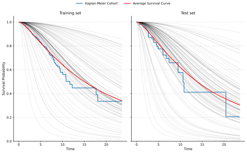
- The theory changes model-selection practice: in-sample AIC/BIC and global deviance are declared invalid for comparing deep distributional architectures, replaced by out-of-sample Anderson-Darling statistics on normalized quantile residuals — with the caveat, in censored survival data, that residual diagnostics be paired with visual checks of predicted survival curves.
- Architecture design follows from the theory: the terminal hidden layer should be an aggressive bottleneck (width M ≤ 4 in the applications), because the second-step parameter count — b + M p_F + p_F — is what determines statistical degrees of freedom and variance inflation.
Reading between the lines
- The intervals in the paper are conditional intervals: they treat the learned features from the first step as fixed, so the honest test of the method is to compare their frequentist coverage with a full two-step bootstrap; the paper's own image experiment (89.35% out-of-sample coverage for nominal 95%) suggests the conditioning gap is material at that scale.
- The width of the terminal bottleneck plays a dual role — representation capacity in step one, statistical degrees of freedom in step two — which points toward a sieve-style asymptotic theory in which M grows slowly with n; that formalization is implicit in the paper but not developed.
- The freeze-and-refit device should transfer to other inference paradigms: Bayesian terminal-layer inference (where the observed Hessian doubles as a Laplace posterior covariance), neural random effects for clustered data, and conformal wraps around the Delta-method intervals as a finite-sample correction.
- A direct calibration experiment is easy to run: simulate from a known GNDR model, refit the full two-step procedure many times, and check whether the inverse observed Hessian tracks the Monte Carlo variance of the terminal-layer estimator — if it does not, the gap identifies exactly where the conditional-normality premise leaks.
Editorial analysis
A structured set of objections, weighed in public.
Referee Report
Summary. The paper introduces Generalized Neural Distributional Regression (GNDR), a two-step estimation framework for parametric distributional regression with deep neural networks. In the first step, the full network (including the terminal layer) is trained by stochastic optimization with early stopping. In the second step, all internal layers are frozen and only the terminal dense layer and classical structured effects are re-estimated by full-data maximum likelihood in a reduced Vector Generalized Linear Model (VGLM). Theorem 1 claims conditional asymptotic normality of this terminal-layer estimator, with covariance given by the inverse Fisher information; the Delta method is then used to build observation-specific confidence bands for distributional parameters, quantiles, and survival curves. The framework is demonstrated on four applications: Dutch boys' BMI with a Box-Cox t distribution, hospital stay counts with a Beta-binomial distribution, TCGA-BRCA survival with various parametric and mixture-cure models, and age prediction from UTKFace images with a zero-truncated normal distribution. The paper also presents the open-source package 'thetaflow'.
Significance. If the conditional-normality claim could be upgraded to a valid unconditional two-step inference statement, GNDR would be a practically valuable bridge between deep representation learning and classical parametric inference, enabling uncertainty quantification on unstructured/high-dimensional data. The manuscript has several strengths: the identifiability discussion is explicit, the reduction to a VGLM is transparent, the Hessian is computed analytically via automatic differentiation, and the authors provide reproducible code and a package. The empirical scope is broad, covering tabular, genomic, and image data. However, the central UQ promise is not yet justified: the asymptotic covariance in Eq. (8) ignores the randomness of the first-step feature extractor, and the model-selection protocol in Section 3.3 makes the reported test-set calibration partly self-referential. These issues are load-bearing for the paper's main claims.
major comments (3)
- [§3.1–3.2, Theorem 1, Eq. (8)] Theorem 1 conditions on v(x)=F_deep(x; \hat\omega_deep), but \hat\omega_deep is estimated from the same training responses and is correlated with the second-step likelihood. The covariance in Eq. (8) is the conditional Fisher information given the realized features, not the total variance of \hat\theta_last or of the Delta-method bands in Eqs. (11)–(16). Standard two-step inference (e.g., Murphy–Topel or Newey–McFadden corrections) is not applied. The empirical test-set coverage of 89.35% in §4.4 is exactly the direction expected from this omission. The manuscript should either provide a corrected covariance that propagates first-step uncertainty, or explicitly reframe the UQ as conditional on the estimated features and temper the coverage claims.
- [§3.3, §4.2, §4.3] The model-selection rule in §3.3 selects the model minimizing the Anderson–Darling statistic on the test set. The applications then report the test-set AD/calibration of the selected model as evidence of 'superior distributional calibration' (e.g., Table 2 and the claim that model (d) 'emerges as the superior architecture'). This is self-referential: the test set is used for selection, so the reported test performance is optimistically biased. A separate validation set for selection, or nested cross-validation, is needed for honest out-of-sample evaluation.
- [Appendix A] The proof of Theorem 1 verifies the VGLM regularity conditions by assertion rather than by argument. In particular, Regularity Condition II requires the concatenated design matrix [z, v(x)] to have full column rank, but v(x)=F_deep(x; \hat\omega_deep) is itself random and estimated, so the fixed-design VGLM conditions of Yee (2015) are not automatically satisfied. The proof also does not clarify the definition of the 'true' θ_last^0 when the feature map is estimated. A rigorous proof requires either an explicit asymptotic framework for the two-step estimator (treating \hat\omega_deep as a nuisance function) or a sample-splitting scheme that makes the feature extractor independent of the second-step likelihood.
minor comments (6)
- [Abstract] Typo: 'packagethetaflow' should read 'package thetaflow'.
- [§2.2] Heading typo: 'identifiabiliy' should be 'identifiability'.
- [Eq. (16)] The notation in (16) writes the limiting distribution as N_p, but f maps R^p to R^q; the dimension should be q or the notation should be clarified.
- [§4.1] The Box-Cox t log-likelihood uses f_T and F_T without explicitly stating that T denotes a Student-t distribution with τ_i degrees of freedom; please define these symbols.
- [Table 3] The 'logit(λ/40)' link for the Cure Mixture Weibull scale imposes an identifiability bound; it would help to state explicitly that this is a modeling assumption and how sensitive results are to the choice of 40.
- [§3.3] The sentence about AIC/BIC being invalid 'except they are comparing the exact same distribution, as it happens in cross validation' is confusing; please clarify the intended scope of the advice.
Circularity Check
Central UQ theory is not circular, but the reported 'superior distributional calibration' is partly self-confirming: the same test-set Anderson–Darling statistic is used both to select the best model and as the evidence that it is best.
-
fitted input called prediction
[Model selection and evaluation: Section 3.3; Section 4.2 (Table 2); Section 4.3 (Table 4)]
"Therefore, when evaluating a set of candidate GNDR architectures or base distributions on the test set, the model minimizing the AD statistic is preferred. ... Based on the out-of-sample evaluation established in Section 3.3, model (d) emerges as the superior architecture, minimizing the AD statistic on the test set. ... Table 4 presents the AD test statistic for each candidate architecture, identifying the Log-logistic distribution as the optimal fit."
The Anderson–Darling statistic on the held-out test set is both the model-selection criterion (Section 3.3: 'the model minimizing the AD statistic is preferred') and the subsequently reported evidence of superiority (Tables 2 and 4, and the surrounding text). Because the chosen model is selected by minimizing exactly this test-set quantity, its top ranking on that same quantity is guaranteed by the selection rule rather than independently confirmed. The test set thus functions as part of the selection procedure, so the empirical claim that the selected GNDR model has superior distributional calibration is partly forced by construction. This does not make Theorem 1 circular, but it weakens the empirical demonstration.
full rationale
The core mathematical derivation is not circular. Theorem 1 explicitly conditions on the frozen latent features v(x), and the proof verifies standard VGLM regularity conditions for the conditional second-step model. Within that conditional model, θ_last is an identifiable parameter, the likelihood is well-defined, and the Fisher information and Delta-method covariance calculations follow from standard asymptotic theory. The fact that v(x) is itself learned from the same responses is a real limitation—the reported intervals are conditional on the fitted feature extractor and omit first-step estimation error, which is consistent with the observed out-of-sample coverage of 89.35%—but it is an incompleteness/statistical weakness, not a circular reduction. The paper also cites prior work for LLLA, neural distributional regression, and VGLMs without relying on a self-citation chain. The only concrete circularity-like step is the empirical model-selection/evaluation loop: the test-set AD statistic is used both to choose the best architecture and as the headline evidence of superior calibration. That step is statistically self-referential and inflates the apparent evidence, but it does not affect the central asymptotic theorem. Accordingly, the overall circularity score is modest.
Assumptions & free parameters
free parameters (7)
- Terminal hidden-layer width M =
1 (hospital), 2 (Dutch boys/survival), 64 (UTKFace)
- Dropout rate =
0.1–0.45 (TCGA), 0.3 (UTKFace)
- Elastic Net L1/L2 penalties =
L1 in {0, 0.0001, 0.0005, 0.1}; L2 in {0.0001, 0.005, 0.01}
- Cure-mixture Weibull scale upper bound =
40
- First-stage epoch/early-stopping schedule =
Not specified
- First hidden-layer width in survival network =
32
- Network topology/activations =
e.g., 24-2 GELU, 24-1 GELU, 32-2 tanh/softplus, MobileNetV2 128/64 GELU
assumptions (7)
- standard math MLE regularity conditions for VGLMs hold for the chosen base distributions and links.
- domain assumption After step 1, v(x) = F_deep(x; ω̂_deep) can be treated as a fixed, known basis expansion.
- domain assumption The augmented design matrix [Z, v(X)] has full column rank.
- domain assumption Neural and classical features feeding the same distributional parameter are disjoint.
- standard math The base distribution D is identifiable and has support independent of parameters.
- ad hoc to paper The bound λ ∈ (0,40) fixes mixture-cure Weibull identifiability.
- domain assumption Selecting the best model by test-set AD statistic leaves an unbiased performance evaluation.
Cite this review
Pith. "Pith review of Generalized Neural Distributional Regression." pith.science (2026). https://pith.science/paper/DDIBRT2A
@misc{pith2026260714122,
  author       = {Pith},
  title        = {Pith review of: Generalized Neural Distributional Regression},
  year         = {2026},
  howpublished = {\url{https://pith.science/paper/DDIBRT2A}},
  note         = {Machine review of arXiv:2607.14122}
}
read the original abstract
We introduce the Generalized Neural Distributional Regression (GNDR) framework, which seamlessly embeds deep neural networks into the parameter space of classical probability distributions. To reconcile the inherent non-identifiability of deep architectures with maximum likelihood theory, we propose a two-step semi-parametric estimation procedure. By isolating the terminal prediction heads and treating the upstream network as a fixed, non-linear basis expansion, GNDR enables the extraction of analytical Fisher Information matrices. This facilitates rigorous uncertainty quantification, generating observation-specific confidence bands and tolerance intervals via the multivariate Delta method. We demonstrate the framework's versatility and superior distributional calibration across diverse data modalities, including overdispersed clinical counts, right-censored transcriptomic survival profiles under a mixture cure framework, and zero-truncated age distributions derived directly from unstructured facial images. The methodology is natively implemented in the open-source Python package \textit{thetaflow}.
Figures


Figures from the paper (7 more)




Reference graph
Works this paper leans on
-
[1]
2014 Fourth international conference on advanced computing & communication technologies , pages=
A detailed review of feature extraction in image processing systems , author=. 2014 Fourth international conference on advanced computing & communication technologies , pages=. 2014 , organization=
2014
-
[2]
Nature Reviews Methods Primers , volume=
Principal component analysis , author=. Nature Reviews Methods Primers , volume=. 2022 , publisher=
2022
-
[3]
Machine learning for data science handbook: data mining and knowledge discovery handbook , pages=
Autoencoders , author=. Machine learning for data science handbook: data mining and knowledge discovery handbook , pages=. 2023 , publisher=
2023
-
[4]
Information fusion , volume=
A review of uncertainty quantification in deep learning: Techniques, applications and challenges , author=. Information fusion , volume=. 2021 , publisher=
2021
-
[5]
ACM Computing Surveys , volume=
A survey on uncertainty quantification methods for deep learning , author=. ACM Computing Surveys , volume=. 2026 , publisher=
2026
-
[6]
, author=
A tutorial on conformal prediction. , author=. Journal of machine learning research , volume=
-
[7]
2012 , publisher=
Bayesian learning for neural networks , author=. 2012 , publisher=
2012
-
[8]
Artificial Intelligence Review , volume=
Deep learning for survival analysis: a review , author=. Artificial Intelligence Review , volume=. 2024 , publisher=
2024
Show all 47 references
-
[9]
ACM Computing Surveys (CSUR) , volume=
Machine learning for survival analysis: A survey , author=. ACM Computing Surveys (CSUR) , volume=. 2019 , publisher=
2019
-
[10]
International Journal of Machine Learning and Cybernetics , volume=
Deep learning for time series forecasting: a survey , author=. International Journal of Machine Learning and Cybernetics , volume=. 2025 , publisher=
2025
-
[11]
Research , volume=
Causal inference meets deep learning: A comprehensive survey , author=. Research , volume=. 2024 , publisher=
2024
-
[12]
IEEE transactions on knowledge and data engineering , volume=
Deep learning for spatio-temporal data mining: A survey , author=. IEEE transactions on knowledge and data engineering , volume=. 2020 , publisher=
2020
-
[13]
Journal of the Royal Statistical Society Series C: Applied Statistics , volume=
Generalized additive models for location, scale and shape , author=. Journal of the Royal Statistical Society Series C: Applied Statistics , volume=. 2005 , publisher=
2005
-
[14]
Computational Statistics & Data Analysis , volume=
Deep distribution regression , author=. Computational Statistics & Data Analysis , volume=. 2021 , publisher=
2021
-
[15]
arXiv preprint arXiv:2010.06889 , year=
Neural mixture distributional regression , author=. arXiv preprint arXiv:2010.06889 , year=
2010 arXiv
-
[16]
2000 , publisher=
Methods of information geometry , author=. 2000 , publisher=
2000
-
[17]
Constructive Approximation , volume=
Neural network identifiability for a family of sigmoidal nonlinearities , author=. Constructive Approximation , volume=. 2022 , publisher=
2022
-
[18]
Neurocomputing , volume=
Structural identifiability of generalized constraint neural network models for nonlinear regression , author=. Neurocomputing , volume=. 2008 , publisher=
2008
-
[19]
NIPS workshop on bayesian deep learning , volume=
Improving the identifiability of neural networks for Bayesian inference , author=. NIPS workshop on bayesian deep learning , volume=
-
[20]
Machine learning , volume=
Parameter identifiability of a deep feedforward ReLU neural network , author=. Machine learning , volume=. 2023 , publisher=
2023
-
[21]
arXiv preprint arXiv:1412.6980 , year=
Adam: A method for stochastic optimization , author=. arXiv preprint arXiv:1412.6980 , year=
-
[22]
arXiv preprint arXiv:1711.05101 , volume=
Fixing weight decay regularization in adam , author=. arXiv preprint arXiv:1711.05101 , volume=
-
[23]
2006 , publisher=
Pattern recognition and machine learning , author=. 2006 , publisher=
2006
-
[24]
Journal of the Royal Statistical Society Series B: Statistical Methodology , volume=
Vector generalized additive models , author=. Journal of the Royal Statistical Society Series B: Statistical Methodology , volume=. 1996 , publisher=
1996
-
[25]
Advances in neural information processing systems , volume=
Laplace redux-effortless bayesian deep learning , author=. Advances in neural information processing systems , volume=
-
[26]
1983 , organization=
Information measures and model selection , author=. 1983 , organization=
1983
-
[27]
Journal of Computational and graphical statistics , volume=
Randomized quantile residuals , author=. Journal of Computational and graphical statistics , volume=. 1996 , publisher=
1996
-
[28]
Statistics in medicine , volume=
Worm plot: a simple diagnostic device for modelling growth reference curves , author=. Statistics in medicine , volume=. 2001 , publisher=
2001
-
[29]
goodness of fit
Asymptotic theory of certain" goodness of fit" criteria based on stochastic processes , author=. The annals of mathematical statistics , pages=. 1952 , publisher=
1952
-
[30]
Statistics in medicine , volume=
On the C-statistics for evaluating overall adequacy of risk prediction procedures with censored survival data , author=. Statistics in medicine , volume=. 2011 , publisher=
2011
-
[31]
Statistical Modelling , volume=
Using the Box-Cox t distribution in GAMLSS to model skewness and kurtosis , author=. Statistical Modelling , volume=. 2006 , publisher=
2006
-
[32]
Journal of the Royal Statistical Society Series C: Applied Statistics , volume=
Use of the beta--binomial distribution to model the effect of policy changes on appropriateness of hospital stays , author=. Journal of the Royal Statistical Society Series C: Applied Statistics , volume=. 1996 , publisher=
1996
-
[33]
PLoS computational biology , volume=
Cox-nnet: an artificial neural network method for prognosis prediction of high-throughput omics data , author=. PLoS computational biology , volume=. 2018 , publisher=
2018
-
[34]
Journal of the royal statistical society: Series B (methodological) , volume=
Regression models and life-tables , author=. Journal of the royal statistical society: Series B (methodological) , volume=. 1972 , publisher=
1972
-
[35]
Journal of the Royal Statistical Society Series B: Statistical Methodology , volume=
Regularization and variable selection via the elastic net , author=. Journal of the Royal Statistical Society Series B: Statistical Methodology , volume=. 2005 , publisher=
2005
-
[36]
Journal of the American Statistical Association , volume=
Survival curve for cancer patients following treatment , author=. Journal of the American Statistical Association , volume=. 1952 , publisher=
1952
-
[37]
Statistics in medicine , volume=
Model diagnostics for censored regression via randomized survival probabilities , author=. Statistics in medicine , volume=. 2021 , publisher=
2021
-
[38]
Statistics in medicine , volume=
Assessment and comparison of prognostic classification schemes for survival data , author=. Statistics in medicine , volume=. 1999 , publisher=
1999
-
[39]
Jama , volume=
Evaluating the yield of medical tests , author=. Jama , volume=. 1982 , publisher=
1982
-
[40]
Nucleic Acids Research , volume=
KEGG: Kyoto Encyclopedia of Genes and Genomes , author=. Nucleic Acids Research , volume=. 2000 , publisher=
2000
-
[41]
Frontiers in Genetics , volume=
Identification and validation of a seven-gene metastasis-associated prognostic model in breast cancer , author=. Frontiers in Genetics , volume=. 2026 , publisher=
2026
-
[42]
MedComm , volume=
Breast Cancer: Molecular Pathogenesis and Targeted Therapy , author=. MedComm , volume=. 2025 , publisher=
2025
-
[43]
International Journal of Medical Science and Clinical Research Studies , volume=
Clinical Applications of Multi-Omics Integration in Disease Diagnosis , author=. International Journal of Medical Science and Clinical Research Studies , volume=. 2026 , doi=
2026
-
[44]
Biomolecules , volume=
Challenges and Opportunities in Multi-Omics Data Acquisition and Analysis: Toward Integrative Solutions , author=. Biomolecules , volume=. 2026 , publisher=
2026
-
[45]
Proceedings of the IEEE International Conference on Computer Vision , pages=
Age progression/regression by conditional adversarial autoencoder , author=. Proceedings of the IEEE International Conference on Computer Vision , pages=
-
[46]
Proceedings of the IEEE conference on computer vision and pattern recognition , pages=
Mobilenetv2: Inverted residuals and linear bottlenecks , author=. Proceedings of the IEEE conference on computer vision and pattern recognition , pages=
-
[47]
2015 , publisher=
Vector generalized linear and additive models: with an implementation in R , author=. 2015 , publisher=
2015
Reviewed August 2, 2026 · model on record in the stance chip above.
Discussion (0). Continue with ORCID to comment.