REVIEW 3 major objections 4 minor 1 cited by
Regularity-Aware Stochastic MGDA with Adaptive Conflict-Avoidant Update Direction Control
T0 review · 3 major / 4 minor · reviewed 2026-08-01 · deepseek-v4-flash
Pith's one-line read Exploiting a hidden Lipschitz regularity speeds stochastic multi-objective learning from O~(T^-1/4) to O~(T^-1/2).
desk verdict The continuity results are real, but the advertised rate improvement comes from the fixed-scalarization fallback, not from the Lipschitz analysis. read the letter →
The pith
A machine-rendered reading of the paper's core claim, the machinery that carries it, and where it could break.
The reading
What carries the argument
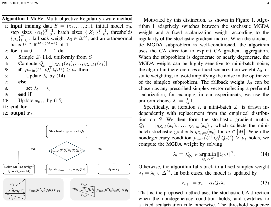
The central object is the conflict-avoidant direction mapping d_Q = -Q λ*_Q, where λ*_Q solves min_{λ∈∆_M} ||Qλ||. The key mechanism is the µ-nondegeneracy condition (Definition 2): with U spanning the simplex tangent space 1^⊥, the matrix U^T Q^T Q U must have smallest eigenvalue ≥ µ, giving strong convexity of the subproblem on the affine hull of the simplex. This forces a unique MGDA weight and yields the Lipschitz bound ||d_{Q1} - d_{Q2}|| ≤ (1 + 2B²/µ) ||Q1 - Q2|| (Lemma 1); absent this condition, only the sharp 1/2-Hölder bound holds (Lemma 2). MoRe (Algorithm 1) turns this into a rule: when µ_min(U^T Q_t^T Q_t U) < µ_t, it replaces the MGDA weight with a fixed scalarization λ_0, prote
What would settle it
A concrete check: implement MoRe on a two-objective quadratic problem whose Hessians are chosen so that the nondegeneracy parameter at the iterates stays above a positive constant, and measure E[min_{t≤T} R_S(x_t)] under the prescribed schedules (|Z_t|=Θ(t+1), α=Θ(T^{-1/2}), µ_t=Θ(1)). If the empirical rate visibly deviates from O(T^{-1/2}) for large T, the claim is false. Conversely, on a problem engineered to approach degeneracy (where the gradients of the two objectives become nearly parallel at the Pareto front), verify that MoRe's rate degrades toward O(T^{-1/4}) as the theory predicts.
Extended reading notes
Core claim
The paper's central discovery is a dichotomy in the continuity of the conflict-avoidant direction map Q ↦ d_Q, where d_Q = -Q λ*_Q is the minimum-norm convex combination of the objective gradients. On any bounded set of gradient matrices, the map is 1/2-Hölder continuous and the exponent 1/2 is sharp (Lemma 2); no higher-order Hölder bound holds in the worst case. But if the reduced curvature matrix U^T Q^T Q U is uniformly lower bounded by µ > 0 (Definition 2), the map is Lipschitz with constant 1 + 2B²/µ (Lemma 1). This regularity gap explains why stochastic MGDA suffers a suboptimal rate, and motivates MoRe, which tests the curvature condition at each step and switches to fixed-scalarizat
Load-bearing premise
The load-bearing premise is Assumption 2: each mini-batch gradient must be unbiased with variance bounded by σ²/|Z_t|, together with Assumption 4's uniform per-sample gradient bound; if gradient noise is heavy-tailed or gradients are unbounded, the Lipschitz-based error control and the improved O~(T^{-1/2}) rate collapse.
Editorial extensions
If this is right
- If the theorem is correct, stochastic multi-objective optimization can match the iteration complexity of single-objective nonconvex SGD (O~(T^{-1/2})), while keeping the conflict-avoidant property of MGDA.
- The per-iterate CA direction distance guarantee gives a quantitative promise that MoRe's updates track the full-batch conflict-avoidant direction, decaying as O(1/log T) under the recommended schedule.
- The threshold µ_t creates an explicit trade-off: larger thresholds give faster convergence, smaller thresholds give better conflict-avoidance; setting µ_t ≈ t^{-1/3} optimizes the CA distance at O(t^{-1/3}).
- The sharpness result (Lemma 2) implies that without a regularity condition or a fallback strategy, no stochastic MGDA variant can achieve linear noise propagation, so the suboptimality of vanilla SMG is intrinsic, not an artifact of the analysis.
Reading between the lines
- Editorial inference: the same regularity-switch principle could improve other nonlinear gradient-aggregation methods (e.g., gradient projection or direction-averaging schemes) that suffer from Hölder-type sensitivity to input noise; the curvature diagnostic is general.
- Editorial inference: the requirement of linearly growing batch sizes is a practical cost; combining MoRe with variance reduction (e.g., multi-objective SVRG) may preserve the O(T^{-1/2}) rate with constant mini-batches, but the paper does not analyze this.
- Editorial inference: the theory concerns the empirical objective; an extension to population-level guarantees (excess risk) would be needed to certify the observed multi-task learning gains beyond the training set.
- Editorial inference: in degenerate regions, MoRe effectively abandons conflict avoidance to preserve stability; an alternative—detecting degeneracy and then increasing batch size—might keep CA behavior without sacrificing the rate, which is a testable variant.
Editorial analysis
A structured set of objections, weighed in public.
Referee Report
Summary. The paper studies the continuity of the MGDA conflict-avoidant (CA) direction map Q -> d_Q in stochastic multi-objective learning. It proves that the map is 1/2-Hölder continuous on bounded sets, with a sharpness example, and that under a μ-nondegeneracy condition (Definition 2) the map is Lipschitz continuous (Lemma 1). Based on this, the authors propose the MoRe algorithm, which switches between the stochastic MGDA direction and a fixed scalarization weight depending on a measured nondegeneracy threshold. Theorem 1 claims a nonconvex Pareto-stationarity rate of O(T^{-1/2}) (tilde-O with a logarithmic threshold schedule) under growing mini-batches |Z_t| = Θ(t+1) and step size α = Θ(T^{-1/2}), compared with the known tilde-O(T^{-1/4}) rate for SMG. Theorem 2 gives a per-iterate CA-direction-distance bound for M=2. Experiments on Office-Home are reported in Table II and Figure 3.
Significance. The continuity analysis in Lemmas 1 and 2 is clean and the sharpness counterexample in Appendix B is explicit and convincing. If the claimed rate were attributable to the Lipschitz mechanism, the paper would be a substantial advance over stochastic MGDA. However, the central attribution is not supported: Theorem 1's convergence rate can be obtained already by the fixed-scalarization fallback in Eq. (70), without any use of Lemma 1, the threshold μ_t, or the switching rule. Thus the claimed rate improvement over SMG does not demonstrate the value of the regularity-aware CA mechanism. The per-iterate CA-distance guarantee in Theorem 2 is a genuine separate contribution, but it is restricted to M=2. The paper's contribution is therefore best described as a fine-grained continuity analysis plus a provably stable fallback schedule, rather than a rate improvement caused by exploiting Lipschitz continuity.
major comments (3)
- [Theorem 1 / Appendix C, Eq. (70)] The claimed convergence-rate improvement is not attributable to the Lipschitz continuity of the CA direction. In Case 2 of the proof, Eq. (70) is exactly the standard scalarized SGD inequality for the fixed weight λ0: α_t R_S(x_t) ≤ λ0^T F_S(x_t) − λ0^T F_S(x_{t+1}) + α_t ℓ_f ||Q_t − ∇F_S(x_t)||_F + O(α_t^2). Summing Eq. (70) over t under |Z_t|=Θ(t+1) and α=Θ(T^{-1/2}) yields E[min_t R_S(x_t)] = O(T^{-1/2}) without ever invoking Lemma 1, the threshold μ_t, or the switching rule. Since R_S(x_t) ≤ ||∇F_S(x_t)λ0||^2, an algorithm that always sets λ_t = λ0 attains the same rate. Therefore the O(T^{-1/2}) rate in Theorem 1 does not support the abstract's claim that exploiting Lipschitz continuity is what enables the improvement over SMG. The paper should either reframe the contribution, or provide a setting where fixed scalarization cannot achieve the rate and the switching mechanism is essen
- [Section IV-B / Figure 3] The empirical section does not discriminate between the proposed mechanism and the trivial always-fallback baseline. Figure 3 only reports the stationarity measure R_S(x_t) with a 1/sqrt(T) reference line; as shown in the major comment above, the always-fixed-scalarization algorithm is also predicted to decay like 1/sqrt(T) under the same schedules. To support the regularity-aware contribution, the experiments should compare MoRe against (a) SMG under the same batch and step schedules, and (b) the always-fallback baseline λ_t = λ0. Reporting the fraction of iterations where the regular branch is used and the per-iterate CA distance would also help verify the switching mechanism.
- [Abstract and Conclusion] The abstract and conclusion state that the method 'exploits the Lipschitz continuity of the CA direction when the subproblem is regular' and thereby 'improves the convergence rate of SMG from tilde-O(T^{-1/4}) to tilde-O(T^{-1/2})'. Given Eq. (70), this causal statement is not established. The rate improvement over SMG is a property of the growing-batch-size fallback to a fixed scalarization, not of the Lipschitz regularity of the CA map. The narrative should be revised so that the convergence-rate claim is decoupled from the Lipschitz-continuity insight; otherwise the central claimed contribution is overstated.
minor comments (4)
- [Assumption 2] The variance bound E||q_{Z_t,m}(x_t) − ∇f_{S,m}(x_t)||^2 ≤ σ^2/|Z_t| is load-bearing for Theorem 1. The Office-Home experiments do not verify this distributional assumption. A brief discussion of the limitation would be appropriate.
- [Theorem 2] The per-iterate CA-distance result is restricted to M=2, and the conclusion acknowledges this. This is fine, but since the paper's broader tables (Table I) highlight only the general convergence rate, the M=2 restriction should be stated more prominently in the abstract or contribution list.
- [Table II] The Office-Home results are reported without standard deviations or multiple-seed information, so it is hard to judge whether the reported improvement over baselines is significant.
- [Appendix C, Eq. (63)] In the regular-branch bound, the indicator 1_{G_t} is dropped to give Eq. (63). This is valid because the term is nonnegative, but the resulting bound is loose. Consider stating explicitly that the price is paid later via the bad-event term.
Circularity Check
Derivation is self-contained; no circularity. The rate theorem is proved from stated assumptions, and self-citations to [2] are not load-bearing.
full rationale
The central derivation chain is not circular. Lemma 1 proves Lipschitz continuity of the CA-direction map from the µ-nondegeneracy condition (Definition 2) using strong convexity of the reduced simplex subproblem; it does not assume the target Lipschitz bound. Lemma 2 proves the 1/2-Hölder bound in-line and establishes sharpness with an explicit two-matrix counterexample whose reduced curvature degenerates as sin^2(t), so it does not rely on the present paper's conclusions. Theorem 1 bounds the Pareto-stationarity measure through a descent inequality on the fixed scalarization λ0, controlling the stochastic direction error with Assumption 2's variance bound and the Lipschitz/bad-event decomposition; the final rate O(T^{-1/2}) under |Z_t|=Θ(t+1), α=Θ(T^{-1/2}) is obtained by summing deterministic inequality terms, not by fitting a constant to data. The proof is valid even if the fixed-scalarization fallback alone would yield a similar rate, as seen in Eq. (70); that is an attribution/ablation concern about which mechanism drives the rate, not a circularity, because the theorem does not assume the CA-direction Lipschitz bound as an input. Theorem 2's per-iterate CA-distance bound follows from a branch decomposition and the M=2 identity µ_min(U^T Q^T Q U)=1/2||q_{Zt,1}-q_{Zt,2}||^2; the manuscript explicitly states the M=2 limitation. Self-citations to [2] (co-authored by L. Chen) are used for definitions of CA-direction distance, baseline method comparisons, and prior rates; the previously established 1/2-Hölder bound is re-derived in Lemma 2 rather than imported, and the claimed O(T^{-1/4}) SMG baseline is an external comparison, not an input to the proof. No parameter is fitted to the target stationarity measure, and no result reduces to its own inputs by construction. Overall, no significant circularity; score 1 reflects only the minor self-citation presence, which is not load-bearing.
Assumptions & free parameters
free parameters (3)
- Regularity threshold schedule μ_t =
Θ(1) or Θ(1/log(e+t)); numerical constants unspecified
- Fallback scalarization weight λ_0 =
Uniform 1/M in experiments; otherwise any fixed simplex vector
- Step size α and batch-size schedule |Z_t| =
α = Θ(T^{-1/2}), |Z_t| = Θ(t+1)
assumptions (6)
- domain assumption Assumption 1: each empirical objective f_{S,m} is bounded below
- domain assumption Assumption 2: unbiased mini-batch gradients with variance ≤ σ²/|Z_t|
- domain assumption Assumption 3: every fixed scalarization λ^T F_S is ℓ_{f,1}-smooth
- domain assumption Assumption 4: bounded per-sample gradients ∥∇f_{z,m}(x)∥ ≤ ℓ_f
- ad hoc to paper μ-nondegeneracy of the stochastic gradient matrix (Definition 2)
- domain assumption Exact solution of the simplex subproblem (14) at every regular-branch iteration
Cite this review
Pith. "Pith review of Regularity-Aware Stochastic MGDA with Adaptive Conflict-Avoidant Update Direction Control." pith.science (2026). https://pith.science/paper/L74XQ4NW
@misc{pith2026260715412,
  author       = {Pith},
  title        = {Pith review of: Regularity-Aware Stochastic MGDA with Adaptive Conflict-Avoidant Update Direction Control},
  year         = {2026},
  howpublished = {\url{https://pith.science/paper/L74XQ4NW}},
  note         = {Machine review of arXiv:2607.15412}
}
abstract
Multi-objective learning (MOL) aims to optimize multiple objectives simultaneously. The multi-gradient descent algorithm (MGDA) is a workhorse that iteratively updates along a common descent or conflict-avoidant (CA) direction across objectives. In stochastic settings, however, the vanilla stochastic MGDA method, SMG, lacks a fast convergence rate because mini-batch sampling introduces noise in the gradients. This causes bias in the update direction, which is controlled by the CA direction continuity. In this paper, we show that the CA direction is $1/2$-Holder continuous with respect to the Jacobian matrix, and the exponent $1/2$ cannot be improved in the worst case. This leads to a suboptimal convergence rate for vanilla stochastic MGDA in prior works. Nevertheless, under additional regularity conditions, we show this can be improved to Lipschitz continuity. Based on this insight, we propose a stochastic multi-objective regularity-aware (MoRe) method that exploits the Lipschitz continuity of the CA direction when the subproblem is regular, and switches to a fixed scalarization weight otherwise. Intuitively, the proposed algorithm employs CA direction update when the gradient conflict is large, and linear scalarization update otherwise. Theoretically, our method improves the convergence rate of SMG in the nonconvex setting from $\widetilde{\mathcal O}(T^{-1/4})$ to $\widetilde{\mathcal O}(T^{-1/2})$, where $\widetilde{\mathcal O}(\cdot)$ hides logarithmic factors. Meanwhile, we also establish the per-iterate conflict-avoidance guarantees. Empirically, experiments demonstrate its effectiveness in multi-task performance and verify convergence behavior consistent with the established theoretical rate.
Figures


Forward citations
Cited by 1 Pith paper
-
Improved Convergence Rate for Stochastic Multi-Gradient Descent: A Proof Discovered with AI
Vanilla stochastic multi-gradient descent achieves Õ(T^{-1}) squared Pareto-stationarity under linearly growing mini-batches, improving the prior Õ(T^{-1/4}) bound.
Reference graph
Works this paper leans on
-
[2]
Three-way trade-off in multi-objective learning: Optimization, generalization and conflict- avoidance,
L. Chen, H. Fernando, Y . Ying, and T. Chen, “Three-way trade-off in multi-objective learning: Optimization, generalization and conflict- avoidance,”Journal of Machine Learning Research, vol. 25, no. 193, pp. 1–53, 2024
2024
-
[12]
The multiobjective steepest descent direction is not Lipschitz continuous, but is H ¨older continuous,
B. F. Svaiter, “The multiobjective steepest descent direction is not Lipschitz continuous, but is H ¨older continuous,”Operations Research Letters, vol. 46, no. 4, pp. 430–433, 2018
2018
-
[1]
The stochastic multi-gradient algorithm for multi-objective optimization and its application to supervised machine learning,
S. Liu and L. N. Vicente, “The stochastic multi-gradient algorithm for multi-objective optimization and its application to supervised machine learning,”Annals of Operations Research, vol. 339, no. 3, pp. 1119– 1148, 2024
2024
-
[3]
Multi-task learning as multi-objective op- timization,
O. Sener and V . Koltun, “Multi-task learning as multi-objective op- timization,” inAdvances in Neural Information Processing Systems, vol. 31, 2018
2018
-
[4]
Multi-objective meta learning,
F. Ye, B. Lin, Z. Yue, P. Guo, Q. Xiao, and Y . Zhang, “Multi-objective meta learning,” inAdvances in Neural Information Processing Systems, vol. 34, 2021, pp. 21 338–21 351
2021
-
[5]
Learning with limited samples: Meta-learning and applications to com- munication systems,
L. Chen, S. T. Jose, I. Nikoloska, S. Park, T. Chen, and O. Simeone, “Learning with limited samples: Meta-learning and applications to com- munication systems,”Foundations and Trends® in Signal Processing, vol. 17, no. 2, pp. 79–208, 2023
2023
-
[6]
Fairness constraints: Mechanisms for fair classification,
M. B. Zafar, I. Valera, M. G. Rogriguez, and K. P. Gummadi, “Fairness constraints: Mechanisms for fair classification,” inProceedings of the 20th International Conference on Artificial Intelligence and Statistics, ser. Proceedings of Machine Learning Research, vol. 54, 20–22 Apr 2017, pp. 962–970
2017
-
[7]
Algorithms for multicriterion optimization,
H. Mukai, “Algorithms for multicriterion optimization,”IEEE Transac- tions on Automatic Control, vol. 25, no. 2, pp. 177–186, 1980
1980
Show all 23 references
-
[8]
Conflict-Averse Gradient Descent for Multi-task Learning,
B. Liu, X. Liu, X. Jin, P. Stone, and Q. Liu, “Conflict-Averse Gradient Descent for Multi-task Learning,” inProc. Advances Neural Inf. Process. Syst., vol. 34, virtual, Dec. 2021, pp. 18 878–18 890. PREPRINT, JULY 2026 7
2021
-
[9]
Steepest descent methods for multicriteria optimization,
J. Fliege and B. F. Svaiter, “Steepest descent methods for multicriteria optimization,”Mathematical methods of operations research, vol. 51, pp. 479–494, 2000
2000
-
[10]
Multiple-gradient descent algorithm (mgda) for multi- objective optimization,
J.-A. D ´esid´eri, “Multiple-gradient descent algorithm (mgda) for multi- objective optimization,”Comptes Rendus. Math ´ematique, vol. 350, no. 5-6, pp. 313–318, 2012
2012
-
[11]
Mitigating gradient bias in multi-objective learning: A prov- ably convergent approach,
H. Fernando, H. Shen, M. Liu, S. Chaudhury, K. Murugesan, and T. Chen, “Mitigating gradient bias in multi-objective learning: A prov- ably convergent approach,” inProc. Int. Conf. Learn. Representations, Kigali, Rwanda, May 2023
2023
-
[13]
Gradient Surgery for Multi-Task Learning,
T. Yu, S. Kumar, A. Gupta, S. Levine, K. Hausman, and C. Finn, “Gradient Surgery for Multi-Task Learning,” inProc. Advances Neural Inf. Process. Syst., vol. 33, virtual, Dec. 2020, pp. 5824–5836
2020
-
[14]
On the convergence of stochastic multi-objective gradient manipulation and beyond,
S. Zhou, W. Zhang, J. Jiang, W. Zhong, J. Gu, and W. Zhu, “On the convergence of stochastic multi-objective gradient manipulation and beyond,” inAdvances in Neural Information Processing Systems, S. Koyejo, S. Mohamed, A. Agarwal, D. Belgrave, K. Cho, and A. Oh, Eds., vol. 35,...
2022
-
[15]
Direction-oriented multi-objective learning: Simple and provable stochastic algorithms,
P. Xiao, H. Ban, and K. Ji, “Direction-oriented multi-objective learning: Simple and provable stochastic algorithms,” inProc. Advances Neural Inf. Process. Syst., vol. 36, New Orleans, LA, USA, 2023, pp. 4509– 4533
2023
-
[16]
FERERO: A flexible framework for preference-guided multi-objective learning,
L. Chen, A. F. M. Saif, Y . Shen, and T. Chen, “FERERO: A flexible framework for preference-guided multi-objective learning,” inProc. Advances Neural Inf. Process. Syst., vol. 37, Vancouver, Canada, 2024, pp. 18 758–18 805
2024
-
[17]
Joint gradient balancing for data ordering in finite-sum multi-objective optimization,
H. Yang and J. T. Kwok, “Joint gradient balancing for data ordering in finite-sum multi-objective optimization,” inProc. Int. Conf. Learn. Representations, Singapore, Apr. 2025
2025
-
[18]
Variance reduction can improve trade-off in multi-objective learning,
H. Fernando, L. Chen, S. Lu, P.-Y . Chen, M. Liu, S. Chaudhury, K. Murugesan, G. Liu, M. Wang, and T. Chen, “Variance reduction can improve trade-off in multi-objective learning,” inProc. IEEE Int. Conf. Acoustics, Speech Signal Process., 2024, pp. 6975–6979
2024
-
[19]
Proximal gradient methods for multiobjective optimization and their applications,
H. Tanabe, E. H. Fukuda, and N. Yamashita, “Proximal gradient methods for multiobjective optimization and their applications,”Computational Optimization and Applications, vol. 72, no. 2, pp. 339–361, 2019
2019
-
[20]
LibMTL: A python library for deep multi-task learning,
B. Lin and Y . Zhang, “LibMTL: A python library for deep multi-task learning,”Journal of Machine Learning Research, vol. 24, no. 209, pp. 1–7, 2023
2023
-
[21]
Deep hashing network for unsupervised domain adaptation,
H. Venkateswara, J. Eusebio, S. Chakraborty, and S. Panchanathan, “Deep hashing network for unsupervised domain adaptation,” inPro- ceedings of the IEEE Conference on Computer Vision and Pattern Recognition, jul 2017, pp. 5018–5027
2017
-
[22]
R. A. Horn and C. R. Johnson,Matrix Analysis, 2nd ed. Cambridge University Press, 2012. PREPRINT, JULY 2026 8 APPENDIX A summary of notation used in this work is listed in Table III for ease of reference. TABLE III NOTATION AND DESCRIPTIONS. Notation Descriptions x∈R p Model p...
2012
-
[23]
Therefore, under the case condition µmin(U ⊤Q⊤ t QtU)< µ t, we have∥q Zt,1 −q Zt,2∥2 <2µ t.Multiplying (93) by1 Rc t , bounding the last term via 1Rc t ∥qZt,1 −q Zt,2∥2 <2µ t, dropping the indicator on the two variance terms, and taking expectations yields E 1Rc t ∥dt −d(x t)∥...
Reviewed August 1, 2026 · model on record in the stance chip above.
Discussion (0). Continue with ORCID to comment.