A Four-Dimensional Gaussian Random Field Generator for Modeling Spatiotemporal Variability in Astrophysical Sources

Alejandro C\'ardenas-Avenda\~no; Diego Rubiera-Garcia; Frederic H. Vincent

REVIEW 3 major objections 3 minor 29 references

A Four-Dimensional Gaussian Random Field Generator for Modeling Spatiotemporal Variability in Astrophysical Sources

T0 review · 3 major / 3 minor · reviewed 2026-08-01 · deepseek-v4-flash

Challenge this review Re-run · record.json Download PDF Read on arXiv ↗

Pith's one-line read A unified semi-analytic prescription gives time-dependent, off-equatorial black-hole source models for ray tracing.

desk verdict A useful, honest 3+1D extension of inoisy with a clean off-equatorial rotation law, but the missing quantitative check of the realized covariance is the gap between plausible and demonstrated. read the letter →

arxiv 2607.16576 v1 pith:7JDWPPLS submitted 2026-07-18 astro-ph.HE astro-ph.IMgr-qc

Alejandro Cárdenas-Avendaño , Diego Rubiera-Garcia , Frederic H. Vincent This is my paper · ORCID

classification astro-ph.HEastro-ph.IMgr-qc

keywords black-holeimagingKerrspacetimeoff-equatorialaccretiondiskGaussianrandomfieldsMatérncovariancestochasticpartialdifferentialequationssourcevariabilityraytracing

verification ladder T0 review T1 audit T2 compute T3 formal

The pith

A machine-rendered reading of the paper's core claim, the machinery that carries it, and where it could break.

The reading

This work unifies two ingredients needed to model black-hole 'movies' without expensive plasma simulations: a prescribed fluid rotation law for a geometrically thick disk in the Kerr spacetime, and a time-dependent stochastic emissivity. The rotation law is a cylindrical angular-momentum profile, lifted from the equatorial plane and normalized by the full Kerr metric at each spacetime point, so that the flow remains timelike throughout the emitting region. The variability is modeled as a four-dimensional inhomogeneous, anisotropic Matérn-like Gaussian random field, whose advection is taken from that same rotation law and whose covariance is a single composite tensor blending torus and jet geometries. If the method performs as intended, a user plugs the given formulas into a ray-tracing pipeline and directly obtains time-dependent thick-disk and disk-jet emission.

What carries the argument

The central object is the local correlation tensor Λ^{ij}(X) = w_d Λ_d^{ij} + w_j Λ_j^{ij}, built as a weighted sum of positive tensors, each assembled from an advection vector and an orthonormal spatial triad with scalar correlation lengths. This composite tensor feeds the anisotropic elliptic operator L = 1 − ∂_i(Λ^{ij}∂_j), which is squared in the four-dimensional Matérn SPDE with ν = 2. The stochastic realization is therefore obtained by solving two second-order elliptic equations on a grid, a computationally tractable step that avoids fractional operators. The load-bearing step is that a finite-grid solve, with periodic time and truncated space, reproduces the intended local covariance

What would settle it

Generate a realization with constant Λ = λ²I on a periodic grid, estimate the realized covariance or power spectrum from the output field, and compare with the analytic Matérn spectrum (1 + λ²k²)^{−4}; a significant mismatch at low or high k, or anisotropic growth near boundaries, would falsify the numerical fidelity claim. For the inhomogeneous case, measure local correlation lengths from multiple realizations inside the torus region and check them against the prescribed λ_d,I.

Watch

Extended reading notes

Core claim

The core claim is that both the mean flow and the flickering can be specified by one closed set of formulas. An off-equatorial Kerr four-velocity is built by lifting an equatorial specific-angular-momentum profile to cylindrical surfaces, setting the polar component to zero, and normalizing with the local Kerr metric; this velocity supplies the advection vector that tilts the stochastic correlations. The random field itself is defined by the SPDE L²F = 4π√6 |Λ|^{1/4} W, where L = 1 − ∂_i(Λ^{ij}∂_j) and Λ is a positive composite tensor formed from weighted disk and jet blocks. Solving this equation with two standard second-order elliptic solves yields a smooth, four-dimensional Matérn-like re

Load-bearing premise

The central premise is that solving the variable-coefficient SPDE on a finite grid with periodic time and truncated space reproduces the intended anisotropic correlation tensor, without boundary or discretization artifacts—this is visually asserted in the paper but never quantitatively verified.

Editorial extensions

If this is right

Users can generate time-dependent, off-equatorial thick-disk and jet emission models by specifying a small set of parameters, without solving the Euler or MHD equations.
The same composite tensor can be reused for polarized radiative coefficients by drawing correlated fluctuations in emissivity, absorptivity, and Faraday rotation.
Statistically independent disk and jet variability can be produced by drawing two Gaussian fields with separate tensors instead of the default composite.
The rotation-law/random-field split allows calibration of correlation lengths and fluctuation amplitudes against simulated or observed black-hole light curves.
The model's variability has a Matérn-type smoothness fixed by ν=2 in four dimensions, implying a concrete power-law falloff that can be checked against generated movies and, after projection, against observed time series.

Reading between the lines

Editorial extensions of the paper, not claims the author makes directly.

The paper provides no quantitative check that the finite-grid SPDE solve actually reproduces the prescribed covariance; a natural next step is to measure realized correlation lengths and power spectra from the output field and compare them with the analytic Matérn prediction.
The cylindrical-lift rotation law, with its timelike-domain checks, stands alone as a convenient kinematic prescription for stationary thick-disk emission, independent of the stochastic part.
The composite tensor could be treated as a prior that is learned from magnetohydrodynamic simulation movies, rather than fixed by hand, allowing the model to match realistic correlation geometry.
The integer-order choice ν=2 is a practical compromise; enabling fractional ν through approximation schemes would produce rougher light curves and could be tested against AGN damped-random-walk observations.

Share X Bluesky LinkedIn Reddit HN

Editorial analysis

A structured set of objections, weighed in public.

Desk editor's note, referee report, and a circularity audit.

Desk Editor's Note

read the letter

Two things to know. First, this is a real step beyond inoisy: a full 3+1D Matérn-type Gaussian random field with a local anisotropic covariance tensor, built as a composite of torus and jet blocks, and coupled to a new, carefully defined off-equatorial Kerr rotation law. Second, the main gap is that the paper never checks that the numerical field actually has the covariance it claims — no empirical correlation lengths, no power spectra, no convergence tests.

What's good: The cylindrical lifting of the equatorial angular-momentum profile is clean; the distinction between the cylindrical radius used to set ℓ and the spacetime point used to normalize the four-velocity is explicit and correct. The composite covariance tensor is positive by construction, and the SPDE factorization with β=2 is internally consistent. The code is public, and the paper is honest about what's phenomenological and what isn't. The timelike-domain checks are at least discussed, and the 'timelike clamp' is a sensible safeguard.

The soft spots, in order of severity. The covariance validation is the big one. The entire output — the Matérn-like scales, the anisotropy, the correlation times — rests on the finite-grid solution of Eq. (18) realizing the intended Λ^ij. That is a load-bearing assumption. With a 33-point stencil, Dirichlet spatial truncation, and periodic time, there are multiple ways for the realized covariance to drift from the local tensor, especially for correlation times comparable to the orbital period in the torus. The paper even states the power spectrum 'can be measured directly' — but does not measure it. That's a one-figure fix, but it's needed.

Second, the claim that δ=3 gives timelikeness for the full |a|<1 range is asserted without proof or a numerical scan. The paper does qualify it, and the clamp helps, but the claim is stronger than what's shown.

Third, the memory footprint — 1.6 TB for the fiducial grid — will limit reproducibility, though the code is public so people can run smaller grids.

These are addressable issues, not fatal flaws. The construction is well-defined and the math is consistent. For a methods paper that is openly a tool, the missing validation is the difference between 'implementation-ready' and 'implemented, untested.' I'd send it to peer review, and ask the authors to add quantitative covariance diagnostics and a timelikeness scan. The paper is worth engaging with; it could become the standard 4D stochastic source model for ray tracing if the checks hold up.

Referee Report

3 major / 3 minor

Summary. The paper proposes a unified semi-analytic prescription for time-dependent thick-disk and disk-jet emission around Kerr black holes. The first ingredient is an off-equatorial, nongeodesic four-velocity field built by lifting an equatorial specific-angular-momentum profile to cylindrical surfaces, setting u^θ=0, and normalizing with the local Kerr metric. The second is a four-dimensional Gaussian random field generated by solving the anisotropic Matérn SPDE L^2 F = noise, with a composite covariance tensor Λ^{ij} that blends torus and jet correlation geometries and is advected by the prescribed velocity field. The authors argue that the resulting model is an implementation-ready source prescription for ray-tracing codes, with a public code released.

Significance. If the construction works as claimed, this would be a valuable tool for generating time-dependent, geometrically thick semi-analytic black-hole images without the cost of GRMHD simulations. The paper's strengths are its explicit algebraic construction, a public code, and a concrete parameter list. The covariance-tensor composition is novel and potentially useful. However, the central quantitative claim—that the finite-grid SPDE solve realizes the intended Matérn-like covariance—is not verified, which limits the current usability of the prescription.

major comments (3)

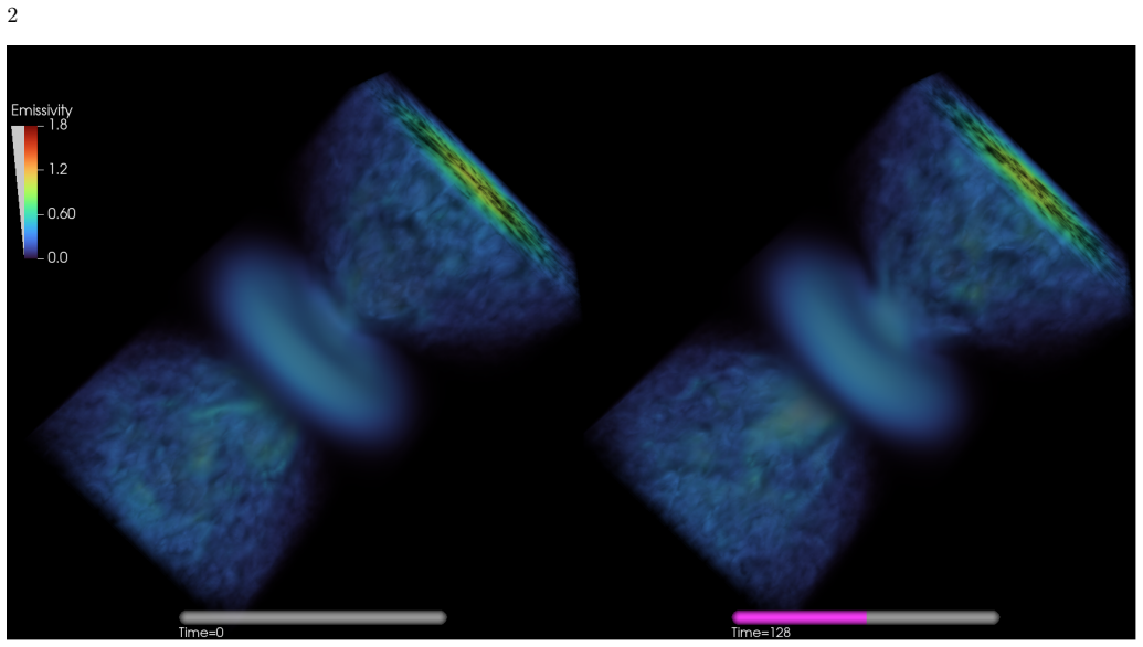
[§3.1–3.3, Eq. (18)–(23), Figs. 1–3] The paper never verifies that the numerical solution of the variable-coefficient SPDE (18) with the composite tensor Λ^{ij} (23) actually yields a Gaussian random field with the prescribed correlation lengths, anisotropy, and temporal behavior. The visual snapshots in Figs. 1 and 3 are not quantitative evidence. The authors even state that the realized power spectrum 'can be measured directly from the generated field' (end of §3.1), but no such measurement is reported. This is load-bearing: the 'Matérn-like' claim and the model's utility for variability studies depend on matching the input correlation scales λ_{α,K} to the output correlations. I request at least one quantitative check: measured correlation lengths along the local triad directions, comparison to the constant-coefficient isotropic analytic spectrum, and a convergence test varying grid spacing and domain size (especially th
[§3.3, boundary conditions] The numerical setup uses homogeneous Dirichlet-type truncation in the spatial directions and periodic time. The paper does not assess boundary or wraparound artifacts, despite the fact that the correlation times (default λ_{d,0}=−1, i.e., orbital time) can be comparable to the 256 M time window. A user following the prescription needs to know whether the fields near the domain edges and near the periodic seam are trustworthy. This is a specific, testable concern: report the empirical autocorrelation in time and space in the interior versus near boundaries, and check that the Dirichlet truncation does not bias the field inside the torus/jet emission region.
[§3.1, Eq. (18)–(19)] The normalization of the SPDE and the subsequent standardization in Eq. (19) are not self-consistent. The paper retains the factor |Λ|^{1/4} from the homogeneous limit, but for a variable-coefficient operator the field variance will not be uniform, so the standardization may introduce non-Gaussianity or hide a mismatch with the intended covariance. The paper does not show the variance map before standardization, nor does it justify that the standardization is a passive rescaling rather than a correction for an unintended inhomogeneity. This again points to the need for a quantitative covariance check.

minor comments (3)

[§3.3, Table 1] The tuple notation for λ_d,A is confusing: the first entry −1 is described as a 'code flag' for using the local orbital time, but later entries are correlation scales. Please separate the flag from the physical parameters or define the tuple explicitly.
[§2, Eq. (5)] The parameters ξ and δ are introduced without physical motivation beyond timelike regularity. A brief discussion of how ξ affects the fluid velocity and whether δ=3 is always safe for the fiducial parameters would help readers who want to vary the rotation law.
[§1 and §3.3] There is an inconsistency in the name: the introduction calls the code 'inoisy+1' while the rest of the paper uses 'inoisy+'. Please standardize.

Circularity Check

0 steps flagged · score 0.0 of 10

No significant circularity: the construction is explicitly phenomenological and all governing equations are defined in the text rather than reduced to prior self-citations.

full rationale

The paper does not claim a first-principles prediction that could collapse into its inputs. Section 1 explicitly disclaims uniqueness: 'Without solving the relativistic Euler or magnetohydrodynamic (MHD) equations ... there is no unique off-equatorial fluid velocity. We therefore adopt a simple stationary and axisymmetric ansatz.' Section 2 then defines the angular-momentum profile by lifting the known equatorial Kerr geodesic expression (Eq. 5) with freely chosen parameters ξ, δ, and Eq. (13) is a constructed four-velocity, not a derived outcome of anything it is later compared with. The stochastic part is the standard SPDE/Matérn factorization (Eqs. 16-18) imported from Lindgren et al. and Lee & Gammie, and the covariance tensor (Eqs. 22-23) with weights (Eqs. 24-27) is a prescribed default from Table 1 whose parameters are inputs, not fitted predictions. The only self-citations (Vincent et al. 2022 for the δ=3 default and radial interpolation, Cárdenas-Avendaño et al. 2023 for the lognormal emissivity) are provenance for openly adopted ansätze or parameter conventions; none is used as a uniqueness theorem or to forbid alternatives. The paper itself says the prescription is 'deliberately phenomenological' and 'does not solve the relativistic Euler equations' (Section 4), which further confirms that no hidden derivation is being claimed. The genuine weakness is that the finite-grid solve of Eq. (18) is not validated against the intended covariance tensor: Section 3.1 only states that its power spectrum 'can be measured directly from the generated field,' and Figs. 1-3 provide visual rather than quantitative support. That is a correctness/validation gap, not circularity, because the realized covariance is not asserted to equal Λ_ij by construction; it is the claim that would need checking.

Assumptions & free parameters 14 free parameters · 6 assumptions · 3 invented entities

The central claim rests on a large set of hand-chosen default parameters (spin, angular-momentum deformation δ, correlation scales, torus/jet geometry) and on domain assumptions about the validity of a u^θ=0 non-geodesic flow law and the fidelity of a finite-grid SPDE solve. No free parameter is fitted to external data; all defaults are modeling choices. No truly new physical entity is introduced—the invented entities are mathematical/modeling constructs with no independent falsifiable handle outside the generated fields.

free parameters (14)

a (Kerr spin) = 0.94
Fiducial source parameter chosen for the example realization; not fitted to data.
σ (angular-momentum branch) = +1 (prograde)
Branch choice in Eq. (5); default is prograde.
ξ = 1
Angular-momentum normalization in Eq. (5); at ξ=1 and δ=0 the equatorial profile reduces to Kerr circular geodesics.
δ = 3.0
Cylindrical angular-momentum deformation; chosen ad hoc to keep the profile timelike down to the horizon. The full-|a|<1 claim is asserted without proof.
β_r = 0.8
Radial interpolation parameter between the orbiting reference flow and zero-angular-momentum free fall in Eq. (11).
λ_d,A = (-1, 5, 1.5, 0.6)
Disk correlation time and surface/meridional/normal scales; -1 is a code flag setting the time scale to the local orbital period.
λ_j,A = (10, 2.5, 2.5, 2.5)
Jet correlation scales: time, helical, polar, and transverse.
R_T, A_T, B_T = (12, 8, 5)
Torus center radius and radial/vertical widths; define the elliptical torus cross-section in Eq. (24).
p = π/20
Disk pitch angle on the torus surface, used in the disk triad of Eq. (26).
R_j,0, α_j = (2.5, 0.30)
Jet core width and opening coefficient in Eq. (27), setting the collimated jet support.
χ0, ρχ = (π/20, 2)
Asymptotic helical angle and axis-regularization scale for the jet triad.
v_j,p, Ω_j = (0.5, 0)
Phenomenological jet advection velocity; not derived from the disk four-velocity.
σ_d, σ_j = (0.2, 0.2)
Lognormal fluctuation amplitudes in Eq. (20); chosen for illustrative snapshots.
ϵ_w = 1e-4
Weight floor added to keep the covariance tensor nonsingular in low-weight regions.

assumptions (6)

standard math The Matérn SPDE representation: solving (1 - ∂Λ∂)^β F = N W produces a Gaussian random field with Matérn-like covariance.
Used in Section 3.1 via Lindgren et al. (2011) and Lee & Gammie (2021).
standard math Kerr metric in Boyer-Lindquist coordinates and the stationary-axisymmetric identities for ℓ(Ω) and Ω(ℓ).
Used throughout Section 2; standard GR identities from Fishbone & Moncrief (1976).
domain assumption Off-equatorial fluid motion can be prescribed by setting u^θ = 0 and assigning angular momentum on cylindrical surfaces, without an explicit pressure or magnetic force model.
Explicitly stated in Section 2: this is a phenomenological force-supported fluid ansatz, not a geodesic or MHD solution.
ad hoc to paper The fiducial δ = 3 choice keeps the angular-momentum profile inside the local timelike domain for the parameter range of interest.
The paper asserts this for the full |a| < 1 when the branch is consistent, but gives no proof; Table 1 also includes a 'timelike clamp'.
domain assumption The finite-difference SPDE solve on a truncated grid with Dirichlet spatial boundaries and periodic time yields the intended inhomogeneous Gaussian random field without significant boundary artifacts.
Central numerical premise of Section 3; the paper provides no quantitative validation of realized covariance.
domain assumption Applying the lognormal transform (20) to the standardized Gaussian field produces a positive emissivity model that preserves the intended spatial and temporal structure.
Adopted in Section 3.1; recognized as a post-processing prescription rather than a radiative-transfer derivation.

invented entities (3)

Cylindrical off-equatorial Kerr rotation law ℓ_{ξ,δ}(ρ)
purpose: Prescribes azimuthal motion of a geometrically thick disk without solving Euler/MHD equations.
Introduced in Eq. (5); a phenomenological fluid ansatz with no falsifiable prediction outside the model.
Composite covariance tensor Λ = w_d Λ_d + w_j Λ_j
purpose: Blends torus and jet variability into a single stochastic field.
Defined in Eq. (23); a model construct that has no independent observable handle outside the generated fields.
Phenomenological jet advection velocity v_j
purpose: Sets the correlation orientation of the jet component.
Default v_j,p = 0.5, Ω_j = 0 in Table 1; explicitly phenomenological and not derived from the disk four-velocity.

how reviews work

0 comments

Cite this review

Pith. "Pith review of A Four-Dimensional Gaussian Random Field Generator for Modeling Spatiotemporal Variability in Astrophysical Sources." pith.science (2026). https://pith.science/paper/7JDWPPLS

@misc{pith2026260716576,
  author       = {Pith},
  title        = {Pith review of: A Four-Dimensional Gaussian Random Field Generator for Modeling Spatiotemporal Variability in Astrophysical Sources},
  year         = {2026},
  howpublished = {\url{https://pith.science/paper/7JDWPPLS}},
  note         = {Machine review of arXiv:2607.16576}
}

read the original abstract

Semi-analytic models of black-hole movies require both an emitting flow prescription and a time-dependent source variability. Existing prescriptions are often limited to either equatorial emission or time-independent sources. In this work we present a unified model for these two ingredients. First, we prescribe an off-equatorial, nongeodesic Kerr fluid rotation law by lifting an equatorial specific-angular-momentum profile to cylindrical surfaces, setting the polar component of the four-velocity to zero, normalizing the flow with the full Kerr metric at the spacetime point, and retaining the option to recover a geodesic-like plunging prescription when needed. Second, we use this velocity as the disk advection field in a four-dimensional inhomogeneous, anisotropic Mat\'ern-like Gaussian random field. We provide a parametrized model for a torus-like disk and a central jet through a single composite correlation tensor. The resulting effective model is an implementation-ready prescription for time-dependent thick-disk and disk-jet emission for relativistic studies.

Figures

Figures reproduced from arXiv: 2607.16576 by the authors.

**Figure 1.** Two snapshots of the positive source field obtained from a single composite torus–jet Gaussian random field using the fiducial values of [PITH_FULL_IMAGE:figures/full_fig_p002_1.png] view at source ↗

**Figure 2.** A torus–jet correlation geometry. The color map shows the unnormalized total weight wd + wj. Top: equatorial xs–ys slice with arrows showing the disk advection velocity vd induced by the normalized Kerr four-velocity. Bottom: meridional xs–zs slice with arrows showing the phenomenological jet advection velocity vj. The figure uses the parameters in [PITH_FULL_IMAGE:figures/full_fig_p007_2.png] view at source ↗

**Figure 3.** Meridional slices through a representative four-dimensional torus–jet realization at ts = 0 and ts = 128. Panels (a) and (b) show the standardized Gaussian random field, Fb(X), at the two epochs, while panels (c) and (d) show the corresponding positive source field, js(X), obtained after applying the envelope and the lognormal mapping of Eq. (20). The imposed envelope makes the thick equatorial torus and the coll… view at source ↗

Discussion (0). Continue with ORCID to comment.

Reference graph

Works this paper leans on

29 extracted references · 6 canonical work pages

[1]

2022, Gaussian Process Regression for Astronomical Time-Series

Aigrain, S., & Foreman-Mackey, D. 2022, Gaussian Process Regression for Astronomical Time-Series. https://arxiv.org/abs/2209.08940

arXiv 2022
[2]

2019, Astrophys

Akiyama, K., et al. 2019, Astrophys. J. Lett., 875, L1, doi: 10.3847/2041-8213/ab0ec7 —. 2022, Astrophys. J. Lett., 930, L12, doi: 10.3847/2041-8213/ac6674

doi:10.3847/2041-8213/ab0ec7 2019
[3]

M., Press, W

Bardeen, J. M., Press, W. H., & Teukolsky, S. A. 1972, ApJ, 178, 347, doi: 10.1086/151796

doi:10.1086/151796 1972
[4]

E., et al

Broderick, A. E., et al. 2020, Astrophys. J., 897, 139, doi: 10.3847/1538-4357/ab91a4

doi:10.3847/1538-4357/ab91a4 2020
[5]

C., Clarkson, C., & Seikel, M

Busti, V. C., Clarkson, C., & Seikel, M. 2014, The Value of H0 from Gaussian Processes. https://arxiv.org/abs/1407.5227 Cárdenas-Avendaño, A., Lupsasca, A., & Zhu, H. 2023, PhRvD, 107, 043030, doi: 10.1103/PhysRevD.107.043030 Cárdenas-Avendaño, A., & Lupsasca, A. 2023, Phys. Rev. D, 108, 064043, doi: 10.1103/PhysRevD.108.064043

arXiv 2014
[6]

D., & Lupsasca, A

Chael, A., Johnson, M. D., & Lupsasca, A. 2021, Astrophys. J., 918, 6, doi: 10.3847/1538-4357/ac09ee

doi:10.3847/1538-4357/ac09ee 2021
[7]

O., Johnson, M

Chang, D. O., Johnson, M. D., Tiede, P., & Palumbo, D. C. M. 2024, Astrophys. J., 974, 143, doi: 10.3847/1538-4357/ad6b28

doi:10.3847/1538-4357/ad6b28 2024
[8]

Cunningham, C. T. 1975, Astrophys. J., 202, 788, doi: 10.1086/154033 da Silva, L. F. D., Lobo, F. S. N., Olmo, G. J., &

doi:10.1086/154033 1975

Show all 29 references

[9]

2023, Phys

Rubiera-Garcia, D. 2023, Phys. Rev. D, 108, 084055, doi: 10.1103/PhysRevD.108.084055

2023 doi
[10]

2019, Physical Review D, 99, 103533, doi: 10.1103/PhysRevD.99.103533

Elizalde, E., & Khurshudyan, M. 2019, Physical Review D, 99, 103533, doi: 10.1103/PhysRevD.99.103533

2019 doi
[11]

2000, Astrophys

Falcke, H., Melia, F., & Agol, E. 2000, Astrophys. J. Lett., 528, L13, doi: 10.1086/312423

2000 doi
[12]

D., Jones, J

Falgout, R. D., Jones, J. E., & Yang, U. M. 2005, ACM Transactions on Mathematical Software, 31, 326

2005
[13]

G., & Moncrief, V

Fishbone, L. G., & Moncrief, V. 1976, ApJ, 207, 962, doi: 10.1086/154565

1976 doi
[14]

Font, J. A. 2008, Living Reviews in Relativity, 11, doi: 10.12942/lrr-2008-7 hypre Developers. 2026,hypre: High Performance

2008 doi
[15]

Preconditioners, Last accessed: 2026-07-17, GitHub, https://github.com/hypre-space/hypre; LLNL, https://computing.llnl.gov/projects/hypre-scalable- linear-solvers-multigrid-methods Ivezić, Ž., & MacLeod, C. L. 2014, in IAU Symposium 304: Multiwavelength AGN Surveys and Studies...

2026 doi
[16]

D., et al

Johnson, M. D., et al. 2020, Sci. Adv., 6, eaaz1310, doi: 10.1126/sciadv.aaz1310 Jordán, A., Eyheramendy, S., & Buchner, J. 2021, State-space Representation of Matérn and Damped Simple Harmonic Oscillator Gaussian Processes. https://arxiv.org/abs/2109.10685

2020 arXiv
[17]

C., Bechtold, J., & Siemiginowska, A

Kelly, B. C., Bechtold, J., & Siemiginowska, A. 2009, The Astrophysical Journal, 698, 895, doi: 10.1088/0004-637X/698/1/895

2009 doi
[18]

2024, Phys

Kocherlakota, P., Rezzolla, L., Roy, R., & Wielgus, M. 2024, Phys. Rev. D, 109, 064064, doi: 10.1103/PhysRevD.109.064064

2024 doi
[19]

Lee, D., & Gammie, C. F. 2021, ApJ, 906, 39, doi: 10.3847/1538-4357/abc8f3

2021 doi
[20]

2011, Journal of the Royal Statistical Society Series B: Statistical Methodology, 73, 423

Lindgren, F., Rue, H., & Lindström, J. 2011, Journal of the Royal Statistical Society Series B: Statistical Methodology, 73, 423

2011
[21]

L., Ivezić, Ž., Kochanek, C

MacLeod, C. L., Ivezić, Ž., Kochanek, C. S., et al. 2010, The Astrophysical Journal, 721, 1014, doi: 10.1088/0004-637X/721/2/1014

2010 doi
[22]

N., Prather, B

Motta, P. N., Prather, B. S., & Cárdenas-Avendaño, A. 2025, Astrophys. J., 995, 56, doi: 10.3847/1538-4357/ae16a0

2025 doi
[23]

Palumbo, D. C. M., Gelles, Z., Tiede, P., et al. 2022, Astrophys. J., 939, 107, doi: 10.3847/1538-4357/ac9ab7

2022 doi
[24]

2016, Astrophys

Pu, H.-Y., Akiyama, K., & Asada, K. 2016, Astrophys. J., 831, 4, doi: 10.3847/0004-637X/831/1/4 Information Systems and Wake Forest University. 2021, WFU High Performance Computing Facility, Wake Forest University, doi: 10.57682/G13Z-2362

2016 doi
[25]

2013, Optimising Gaussian Processes for Reconstructing Dark Energy Dynamics from Supernovae

Seikel, M., & Clarkson, C. 2013, Optimising Gaussian Processes for Reconstructing Dark Energy Dynamics from Supernovae. https://arxiv.org/abs/1311.6678

2013 arXiv
[26]

2025, Astron

Perrin, G. 2025, Astron. Astrophys., 700, A193, doi: 10.1051/0004-6361/202554919

2025 doi
[27]

H., Gralla, S

Vincent, F. H., Gralla, S. E., Lupsasca, A., & Wielgus, M. 2022, A&A, 667, A170, doi: 10.1051/0004-6361/202244339 11

2022 doi
[28]

H., Paumard, T., Gourgoulhon, E., & Perrin, G

Vincent, F. H., Paumard, T., Gourgoulhon, E., & Perrin, G. 2011, Class. Quant. Grav., 28, 225011, doi: 10.1088/0264-9381/28/22/225011

2011 doi
[29]

N., et al

Wong, G. N., et al. 2022, Astrophys. J. Supp., 259, 64, doi: 10.3847/1538-4365/ac582e

2022 doi

Pith tools

Reviewed August 1, 2026 · model on record in the stance chip above.

[1] [1]

2022, Gaussian Process Regression for Astronomical Time-Series

Aigrain, S., & Foreman-Mackey, D. 2022, Gaussian Process Regression for Astronomical Time-Series. https://arxiv.org/abs/2209.08940

arXiv 2022

[2] [2]

2019, Astrophys

Akiyama, K., et al. 2019, Astrophys. J. Lett., 875, L1, doi: 10.3847/2041-8213/ab0ec7 —. 2022, Astrophys. J. Lett., 930, L12, doi: 10.3847/2041-8213/ac6674

doi:10.3847/2041-8213/ab0ec7 2019

[3] [3]

M., Press, W

Bardeen, J. M., Press, W. H., & Teukolsky, S. A. 1972, ApJ, 178, 347, doi: 10.1086/151796

doi:10.1086/151796 1972

[4] [4]

E., et al

Broderick, A. E., et al. 2020, Astrophys. J., 897, 139, doi: 10.3847/1538-4357/ab91a4

doi:10.3847/1538-4357/ab91a4 2020

[5] [5]

C., Clarkson, C., & Seikel, M

Busti, V. C., Clarkson, C., & Seikel, M. 2014, The Value of H0 from Gaussian Processes. https://arxiv.org/abs/1407.5227 Cárdenas-Avendaño, A., Lupsasca, A., & Zhu, H. 2023, PhRvD, 107, 043030, doi: 10.1103/PhysRevD.107.043030 Cárdenas-Avendaño, A., & Lupsasca, A. 2023, Phys. Rev. D, 108, 064043, doi: 10.1103/PhysRevD.108.064043

arXiv 2014

[6] [6]

D., & Lupsasca, A

Chael, A., Johnson, M. D., & Lupsasca, A. 2021, Astrophys. J., 918, 6, doi: 10.3847/1538-4357/ac09ee

doi:10.3847/1538-4357/ac09ee 2021

[7] [7]

O., Johnson, M

Chang, D. O., Johnson, M. D., Tiede, P., & Palumbo, D. C. M. 2024, Astrophys. J., 974, 143, doi: 10.3847/1538-4357/ad6b28

doi:10.3847/1538-4357/ad6b28 2024

[8] [8]

Cunningham, C. T. 1975, Astrophys. J., 202, 788, doi: 10.1086/154033 da Silva, L. F. D., Lobo, F. S. N., Olmo, G. J., &

doi:10.1086/154033 1975