REVIEW 4 major objections 5 minor 297 references
Signed distance to a point cloud can be computed by blending locally fitted tori, pointwise and fast, with no global solves or meshing.
Reviewed by Pith at T0; open to challenge. T0 means a machine referee read the full paper against a public rubric. the ladder, T0–T4 →
T0 review · deepseek-v4-flash
2026-08-01 19:28 UTC pith:WTEB4RLO
load-bearing objection Clever and practical point-cloud SDF method with a nice theoretical frame, but the learned coefficients are the load-bearing part and they demonstrably choke on denser samplings. the 4 major comments →
Points as Tori: Fast Pointwise Signed Distance for Point Clouds
The pith
A machine-rendered reading of the paper's core claim, the machinery that carries it, and where it could break.
Core claim
The paper's central claim is that the self-normalized exponential blend of per-point torus SDFs (Algorithm 1 / Eq. 25) approximates the signed distance to the surface underlying a point cloud, simultaneously reconstructing the surface as the zero level set and providing distance elsewhere. The authors show analytically that among convolutional distance formulas only the self-normalized form (Eq. 17) can avoid the fundamental limitation of 'snapping' to the sampled points, provided the per-point functions carry second-order surface information; tori are chosen because their SDFs are closed form and they reproduce up to second-order local geometry. The torus parameters come from a small pre-tr
What carries the argument
The central object is the self-normalized convolutional distance formula (Eq. 17, evaluated in shifted form Eq. 25): a kernel-density average of per-point functions g_i weighted by exp(-lambda |x-p_i|), which by Laplace's method converges to the value of g at the closest point as lambda grows. The blended functions g_i are SDFs of tori fitted to each point via six learned polynomial coefficients (shift, first/second fundamental forms), chosen so the torus equator passes through the shifted point with matching principal curvatures. The theoretical load-bearing piece is the signed Hopf-Cole transformation, which turns the viscous eikonal equation into a jump screened Laplace equation and shows
Load-bearing premise
The whole method hinges on the pre-trained network's torus coefficients transferring to unseen sampling conditions—density, noise, holes, topology—since the blend just interpolates whatever per-point functions it is given.
What would settle it
Take a point cloud whose sampling density is well outside the training range (e.g., 10x denser with strong noise), fit tori, and compare the zero level set and SDF gradient norms against ground truth on a shape with known SDF. If the level sets deviate systematically while a classical local fit (e.g., tuned weighted least squares quadratic) stays accurate, the learned coefficients, not the blending formula, are the cause; the paper's Fig. 29 already hints at such a failure mode.
If this is right
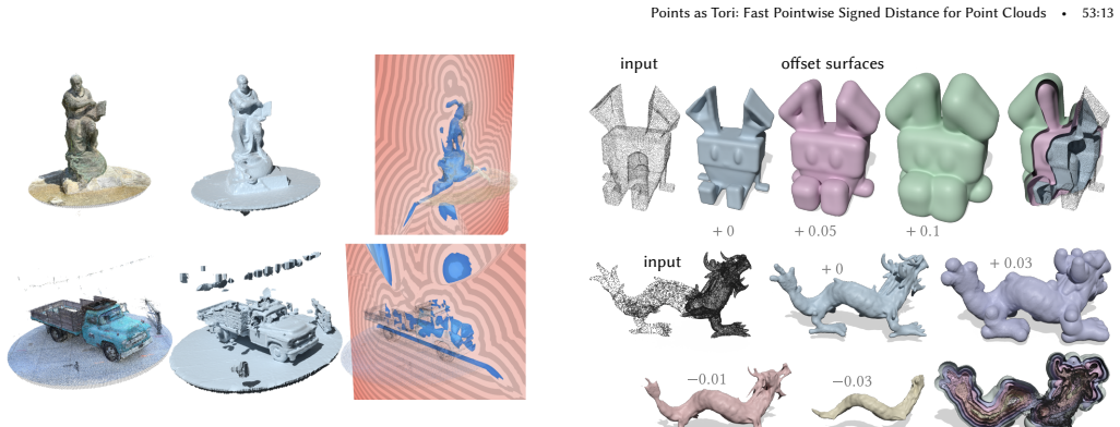
- Point clouds with normals become directly usable in SDF-based pipelines: offsets, Booleans, morphological dilation/erosion, and sphere tracing, with no intermediate mesh.
- The method is output-sensitive: query cost is roughly 10^-4 to 10^-3 seconds per point on million-point clouds, and evaluations parallelize, making per-query distance feasible at arbitrary resolution.
- The theory places winding numbers and Poisson surface reconstruction as limiting cases (screening parameter -> 0) of the same screened-Laplace formulation, so signed distance, occupancy, and reconstruction are unified in one framework.
- Robustness to noise, outliers, uneven sampling, and inconsistently oriented normals is claimed, including an optional iterative orientation procedure driven by SDF gradients.
Where Pith is reading between the lines
- If the blend is as robust as claimed, the representation is a natural differentiable shape proxy for inverse rendering and optimization: because tori are analytic, gradients of the SDF flow through the network outputs, so point clouds could be optimized directly as shape parameters.
- The theory suggests a testable equivalence: for closed clean geometry, tuning the screening parameter lambda should interpolate continuously between winding-number-style occupancy (lambda small) and true distance (lambda large); checking this on a known shape would separate the theory from the learned torus fitting.
- The learned-coefficient bottleneck could be replaced: if a non-learned, robust torus-fitting scheme were developed, the method's generality and failure modes would change; the paper itself flags this as future work.
- Sampling density is a known weak spot (the paper's Fig. 29 shows interior SDF can worsen as sampling densifies); a denser-trained variant or adaptive neighborhood sizing would be a direct extension.
Editorial analysis
A structured set of objections, weighed in public.
Referee Report
Summary. The paper introduces “Points as Tori” (PAT), a method for computing signed distance to an oriented point cloud without global optimization or spatial discretization. For each input point, a pre-trained transformer predicts six polynomial coefficients of a local surface patch; these coefficients determine a fitted torus with a closed-form SDF. The global SDF is then the exponentially weighted, self-normalized blend of per-point torus SDFs (Eq. 1 / Algorithm 1, evaluated as Eq. 25). The theoretical part derives convolutional distance formulas from a signed Hopf–Cole transformation, connects them to winding numbers, Poisson surface reconstruction, and other classic methods, and argues that only the self-normalized formula (Eq. 17) is viable for point clouds. Experiments show fast pointwise queries on clouds up to 29M points, qualitative reconstructions from photogrammetry and other sources, and competitive accuracy on sparse (512-point) datasets. The paper is clearly written and contains substantial theoretical and algorithmic content.
Significance. If the central claim holds—that a pre-trained network can produce per-point torus coefficients that generalize to unseen point clouds and yield a faithful SDF—PAT would be a significant contribution: it offers an output-sensitive, parallelizable, differentiable SDF representation for point clouds, avoiding per-shape fitting and global solves. The theoretical unification of signed distance with winding numbers and Poisson surface reconstruction is elegant and of independent interest. The paper also makes a credible case that the learned component is minimal, with the hard global problem handled by the analytical blend. However, the central accuracy claim is currently conditional: the paper’s own experiments show that density changes degrade the interior SDF (Fig. 29), and the evaluation does not quantitatively cover the density, noise, hole, and topology variation that real point clouds exhibit. The omission of area weights in Eq. 25 is defended only by a hypothesis. These issues are load-bearing for the advertised scope, though they may be addressable with additional experiments, adaptive mechanisms, or a narrowed claim.
major comments (4)
- [§6, Fig. 29] The central claim is that PAT “infers signed distance to a well-reconstructed surface underlying imperfect observations.” Yet the paper states in Section 6 and shows in Fig. 29 that as sampling density increases from 110k to 29M points, the interior SDF “can paradoxically get worse,” with the hypothesized cause being that fixed k=64 neighborhoods shrink and the network fits “compact tori.” This is a direct failure mode for a major class of inputs—dense point clouds—which are precisely the inputs used in the performance demonstrations (Figs. 16, 20, 21). The paper offers only a hypothesis and future-work suggestions. To support the central claim, the authors must either demonstrate that accuracy is maintained across densities, or provide a mechanism (e.g., density-adaptive k, λ, or subsampling) that makes the method robust, or explicitly narrow the claim to a restricted density range. The
- [§4.2, Eq. (25)] Equation (17) is a surface integral with respect to area measure dA. Its discretization in Eq. (25) sums over points without area weights. For non-uniform point clouds—which appear throughout the applications (COLMAP, GLOMAP, uneven sampling in Fig. 22)—omitting area weights biases the exponential average toward densely sampled regions. The paper’s sole justification is the sentence “We hypothesize that we do not observe many ill effects because we fit surfaces with area, rather than singular kernels.” This is an untested hypothesis. Since the method is explicitly aimed at imperfect, non-uniform observations, this is a load-bearing assumption. The authors should either include area weights (computed as in their SSPD baseline) or provide quantitative evidence that their omission does not materially bias the SDF on non-uniform clouds. Without this, the accuracy of the method on real scanne
- [§4.3 / §5.2] The network is trained on point clouds of roughly 2048 points with k=64, and the main quantitative evaluation uses 512-point uniformly sampled point clouds. The paper does not report quantitative accuracy as a function of density, noise level, hole size, or topology. The qualitative demonstrations on dense, noisy, and incomplete data are encouraging, but they do not measure error against ground truth. Given that the central claim depends on the pre-trained network’s generalization, the evaluation needs a systematic study: vary sampling density (e.g., 512, 2048, 8k, 64k, 1M), add noise and outliers, and measure SDF error on the same benchmarks. Without such a study, the reader cannot tell whether the method is broadly applicable or only works near the training distribution. The paper’s own Section 6 acknowledges that “predictions might not be robust for point clouds whose sampling charact
- [§4.2, lambda heuristic] The paper sets λ via the heuristic λ=10^3/D, where D is the mean distance to the 64 nearest neighbors averaged over the cloud, and then R_eval=2C/λ. This is a global, hand-set rule that is not adapted to local density or noise. Since λ controls the effective blending radius, the same λ may be inappropriate for clouds with varying density or noise (as Fig. 30 suggests). The paper states that “sophisticated tuning” is left to future work. While this is not itself an error, it interacts with the density-generalization problem: a failure at high density could be due to the network, the fixed k, or the λ heuristic, and the current evaluation cannot separate these. At minimum, the authors should report sensitivity of their results to λ and to the choice of k, or provide a principled procedure for setting these parameters on a new cloud. This is needed to make the claimed “fast and parameter-li
minor comments (5)
- [§4.2] The relationship between λ_x in Eq. (26) and the heuristic λ=10^3/D used for the radius R_eval is not fully clarified. Are these the same λ used in Eq. (25)? The text jumps between the formula’s shifted exponent and the acceleration heuristic; please define both and state which one is used in the final SDF evaluation.
- [Eq. (15)] Equation (15) uses det(∇²φ(x*)) without stating the assumption that x* is a non-degenerate minimizer with positive-definite Hessian. This is standard for Laplace’s method, but a sentence or footnote would help readers apply the formula to Eq. (17).
- [Figures 16, 20] The captions for Figures 16 and 20 say “Query: s” with the numeric value apparently missing or lost in formatting. Since query time is a central performance claim, the actual values should appear in the figure or caption.
- [Appendix A.1] The open-surface case introduces the ansatz sign_Ω = sign_w. This is a legitimate derivation step, but the main text (Section 2.1) may overstate the validity of the signed Hopf–Cole transformation for open surfaces. Consider adding a forward reference to Appendix A.1 clarifying that this is an assumption, not a theorem, for non-closed geometry.
- [§5.2] The evaluation reports mean absolute error on a 64^3 grid. This global average can be dominated by far-field behavior. Reporting near-surface errors (e.g., within a band around the zero set) would better reflect reconstruction quality and SDF usability for offsets and Boolean operations.
Circularity Check
No significant circularity: the asymptotic derivation is self-contained, and the learned torus fitting is disclosed supervised regression evaluated on held-out data.
full rationale
The paper's claimed derivation chain is not circular. Section 2 derives the self-normalized convolutional formula (Eq. 17) from Green's function and Laplace's method, with the signed Hopf-Cole transformation re-derived in Appendix A and relying on the external result of Lipman (2021) rather than on the present authors' prior work. The algorithm instantiates Eq. 17 with per-point torus SDFs, and the torus parameters are produced by a neural network trained with an explicitly stated loss (Eq. 27) against ground-truth SDFs on ABC and procedurally generated shapes. This is ordinary supervised fitting: the fitted parameters are not calibrated on the evaluation data, and the reported accuracy is measured on held-out shapes (Section 5.2). The paper's own limitation statements (Section 6, Figs. 28–29) acknowledge that predictions may degrade for sampling densities far from the training distribution, and that Eq. 25 omits area weights; these are generalization and approximation concerns, not steps that reduce the output to its inputs by construction. Self-citations such as Feng et al. (2023) for jump harmonic functions and Feng and Crane (2024) as a baseline are contextual and not load-bearing for the central algorithmic claim. Therefore no equation or fitted quantity is equivalent to the claimed result by definition, and the central derivation retains independent mathematical and empirical content.
Axiom & Free-Parameter Ledger
free parameters (5)
- Neural network weights =
trained on ~12k shapes (ABC + procedural blobs)
- lambda scale constant =
1000
- C (exponent precision constant) =
64
- Neighborhood size k =
64
- Loss weighting and query sampling =
equal distance/eikonal weights; 1/3 uniform, 1/3 narrow band, 1/3 cube
axioms (6)
- standard math Laplace's method asymptotic expansion (Eq. 15) with a unique minimizer x*
- domain assumption Point cloud is sampled from a smooth-enough surface so each local neighborhood is well approximated by a torus (second-order proxy)
- domain assumption Input point cloud comes with normals that are (mostly) consistently oriented; torus sign follows normal orientation (Eq. 22)
- ad hoc to paper Area weights in the discretized surface integral (Eq. 17) can be omitted without materially biasing the SDF
- ad hoc to paper Open-surface ansatz sign_Omega = sign w in the signed Hopf-Cole transformation
- standard math The torus SDF formula in Eq. 23 (distance to the center circle minus minor radius) is the exact signed distance of a solid torus
read the original abstract
We describe a method for computing signed distance to point clouds that allows fast pointwise evaluation at arbitrary spatial resolution. As input, our method takes a point cloud with normals; as output, it provides an analytical parameterization that allows queries of signed distance to the approximate underlying surface at arbitrary points - simultaneously providing reconstruction and distance. Our key idea is to reconstruct shapes by locally fitting point clouds with tori, which have closed-form signed distance functions. Tori are fitted in a feed-forward manner, using a pre-trained network to output per-point curvature and shift parameters. Importantly, our method does not require costly global optimization or spatial discretization, and is easily parallelizable. Underlying our method is a new theory that unifies signed distance with the classic reconstruction methods of winding numbers and Poisson surface reconstruction. We use our method to compute signed distance to point clouds arising from photogrammetry, meshes, 3D Gaussians, and neural implicits. Our method allows point clouds to be used directly in applications, without explicit surface reconstruction: as examples, we take offsets of point clouds, apply morphological and Boolean operations, and directly visualize offset surfaces using sphere tracing.
Figures




Reference graph
Works this paper leans on
-
[1]
ACM Transactions on Graphics (TOG) , volume=
Geodesics in heat: A new approach to computing distance based on heat flow , author=. ACM Transactions on Graphics (TOG) , volume=. 2013 , publisher=
2013
-
[2]
ACM Trans
Sharp, Nicholas and Soliman, Yousuf and Crane, Keenan , title =. ACM Trans. Graph. , volume =. 2019 , publisher =
2019
-
[3]
The Discrete Geodesic Problem , author=. SIAM J. Comput. , year=
-
[4]
Surazhsky, Vitaly and Surazhsky, Tatiana and Kirsanov, Danil and Gortler, Steven J. and Hoppe, Hugues , title =. ACM Trans. Graph. , month = jul, pages =. 2005 , issue_date =. doi:10.1145/1073204.1073228 , abstract =
arXiv 2005
-
[5]
, author =
Accurate Computation of Geodesic Distance Fields for Polygonal Curves on Triangle Meshes. , author =. VMV , year =
-
[6]
ACM Trans
Sharp, Nicholas and Crane, Keenan , title =. ACM Trans. Graph. , volume =. 2020 , publisher =
2020
-
[7]
Computer Graphics Forum , title =
Stein, Oded and Wardetzky, Max and Jacobson, Alec and Grinspun, Eitan , year =. Computer Graphics Forum , title =
-
[8]
Computer Graphics Forum , volume=
SSD: Smooth Signed Distance Surface Reconstruction , author=. Computer Graphics Forum , volume=. 2011 , organization=
2011
-
[9]
Proceedings of the National Academy of Sciences , volume =
James A Sethian , title =. Proceedings of the National Academy of Sciences , volume =. 1996 , doi =. https://www.pnas.org/doi/pdf/10.1073/pnas.93.4.1591 , abstract =
-
[10]
ACM Trans
Alec Jacobson and Ladislav Kavan and Olga Sorkine , title =. ACM Trans. Graph. , volume =
-
[11]
1990 , publisher=
Kravtsov, Yury Aleksandrovich and Orlov, Yury Ilich , volume=. 1990 , publisher=
1990
-
[12]
2018 , journal =
Fast Winding Numbers for Soups and Clouds , author =. 2018 , journal =
2018
-
[13]
and Cohen-Steiner, D
Alliez, P. and Cohen-Steiner, D. and Tong, Y. and Desbrun, M. , title =. Proceedings of the Fifth Eurographics Symposium on Geometry Processing , pages =. 2007 , isbn =
2007
-
[14]
Computer Graphics Forum , volume =
Mullen, Patrick and De Goes, Fernando and Desbrun, Mathieu and Cohen-Steiner, David and Alliez, Pierre , title =. Computer Graphics Forum , volume =. doi:10.1111/j.1467-8659.2010.01782.x , year =
arXiv 2010
-
[15]
Proceedings of the IEEE/CVF Conference on Computer Vision and Pattern Recognition (CVPR) , month =
Park, Jeong Joon and Florence, Peter and Straub, Julian and Newcombe, Richard and Lovegrove, Steven , title =. Proceedings of the IEEE/CVF Conference on Computer Vision and Pattern Recognition (CVPR) , month =
-
[16]
Amos Gropp and Lior Yariv and Niv Haim and Matan Atzmon and Yaron Lipman , title =. CoRR , volume =. 2020 , url =. 2002.10099 , timestamp =
Pith/arXiv arXiv 2020
-
[17]
Hoppe, Hugues and DeRose, Tony and Duchamp, Tom and McDonald, John and Stuetzle, Werner , title =. 1992 , issue_date =. doi:10.1145/142920.134011 , journal =
arXiv 1992
-
[18]
Extraction of Shape Skeletons from Grayscale Images , journal =. 1997 , issn =. doi:10.1006/cviu.1997.0612 , author =
arXiv 1997
-
[19]
Curless, Brian and Levoy, Marc , title =. 1996 , isbn =. doi:10.1145/237170.237269 , booktitle =
arXiv 1996
-
[20]
Discrete Quadratic Curvature Energies , year =
Wardetzky, Max and Bergou, Mikl\'. Discrete Quadratic Curvature Energies , year =. Comput. Aided Geom. Des. , month =. doi:10.1016/j.cagd.2007.07.006 , abstract =
-
[21]
Identifying Vector Field Singularities Using a Discrete Hodge Decomposition
Polthier, Konrad and Preu , Eike. Identifying Vector Field Singularities Using a Discrete Hodge Decomposition. Visualization and Mathematics III. 2003
2003
-
[22]
Stein, Oded and Grinspun, Eitan and Wardetzky, Max and Jacobson, Alec , title =. ACM Trans. Graph. , issue_date =. 2018 , issn =. doi:10.1145/3186564 , acmid =
- [23]
-
[24]
Alec Jacobson and Daniele Panozzo and others , note =
-
[25]
CGAL User and Reference Manual
The CGAL Project. CGAL User and Reference Manual
-
[26]
R. Anderson and J. Andrej and A. Barker and J. Bramwell and J.-S. Camier and J. Cerveny V. Dobrev and Y. Dudouit and A. Fisher and Tz. Kolev and W. Pazner and M. Stowell and V. Tomov and I. Akkerman and J. Dahm and D. Medina and S. Zampini , journal =. doi:10.1016/j.camwa.2020.06.009 , volume =
-
[27]
Matan Atzmon and Yaron Lipman , title =. CoRR , volume =. 2019 , url =. 1911.10414 , timestamp =
Pith/arXiv arXiv 2019
-
[28]
2020 , eprint=
SALD: Sign Agnostic Learning with Derivatives , author=. 2020 , eprint=
2020
-
[29]
, author=
A fast marching level set method for monotonically advancing fronts. , author=. proceedings of the National Academy of Sciences , volume=. 1996 , publisher=
1996
- [30]
-
[31]
Carr, Jonathan C. and Beatson, Rick K. and Cherrie, J. B. and Mitchell, T. J. and Fright, W Richard and McCallum, Bruce C. and Evans, T. R. , title =. Proceedings of the 28th Annual Conference on Computer Graphics and Interactive Techniques , pages =. 2001 , isbn =. doi:10.1145/383259.383266 , abstract =
arXiv 2001
- [32]
-
[33]
Variational implicit surfaces , author=
-
[35]
ACM SIGGRAPH 2005 Courses , pages =
Ohtake, Yutaka and Belyaev, Alexander and Alexa, Marc and Turk, Greg and Seidel, Hans-Peter , title =. ACM SIGGRAPH 2005 Courses , pages =. 2005 , isbn =. doi:10.1145/1198555.1198649 , abstract =
arXiv 2005
-
[36]
A multi-scale approach to 3D scattered data interpolation with compactly supported basis functions , year=
Ohtake, Yutaka and Belyaev, Alexander and Seidel, Hans-Peter , booktitle=. A multi-scale approach to 3D scattered data interpolation with compactly supported basis functions , year=
- [37]
-
[38]
Feng, Nicole and Gillespie, Mark and Crane, Keenan , title =. 2023 , issue_date =. doi:10.1145/3592401 , journal =
-
[40]
IEEE Transactions on Visualization and Computer Graphics , year =
Mancinelli, Claudio and Nazzaro, Giacomo and Pellacini, Fabio and Puppo, Enrico , title =. IEEE Transactions on Visualization and Computer Graphics , year =
-
[41]
ACM Transactions on Graphics , year =
Nazzaro, Giacomo and Puppo, Enrico and Pellacini, Fabio , title =. ACM Transactions on Graphics , year =
-
[42]
DGtal: Digital Geometry tools and algorithms library , author =
-
[43]
VolGallery , author =
-
[44]
Heat Kernels and Dirac Operators , year =
Berline, Nicole and Getzler, Ezra and Vergne, Mich\`. Heat Kernels and Dirac Operators , year =
-
[45]
ACM Trans
Sawhney, Rohan and Crane, Keenan , title =. ACM Trans. Graph. , volume =. 2020 , publisher =
2020
-
[46]
ACM Trans
Sawhney, Rohan and Seyb, Dario and Jarosz, Wojciech and Crane, Keenan , title =. ACM Trans. Graph. , volume =. 2022 , publisher =
2022
-
[47]
ACM Trans
Miller, Bailey and Sawhney, Rohan and Crane, Keenan and Gkioulekas, Ioannis , title =. ACM Trans. Graph. , volume =. 2023 , publisher =
2023
-
[48]
ACM Trans
Sawhney, Rohan and Miller, Bailey and Gkioulekas, Ioannis and Crane, Keenan , title =. ACM Trans. Graph. , volume =. 2023 , publisher =
2023
-
[49]
ACM Trans
A Practical Walk-on-Boundary Method for Boundary Value Problems , author =. ACM Trans. Graph. , month =. 2023 , issue_date =
2023
-
[50]
Ronald R. Coifman and St\'. Diffusion maps , journal =. 2006 , note =. doi:10.1016/j.acha.2006.04.006 , url =
-
[51]
Computer Graphics Forum , volume =
Herholz, Philipp and Alexa, Marc , title =. Computer Graphics Forum , volume =. doi:10.1111/cgf.13607 , year =
-
[52]
arXiv e-prints , keywords =
A Survey of Algorithms for Geodesic Paths and Distances. arXiv e-prints , keywords =
-
[53]
ACM Trans
Gillespie, Mark and Sharp, Nicholas and Crane, Keenan , title =. ACM Trans. Graph. , volume =. 2021 , publisher =
2021
-
[54]
Liu, Hsueh-Ti Derek and Gillespie, Mark and Chislett, Benjamin and Sharp, Nicholas and Jacobson, Alec and Crane, Keenan , title =. ACM Trans. Graph. , volume =. 2023 , publisher =. doi:10.1145/3592403 , month =
-
[55]
Journal of computational physics , volume=
A variational level set approach to multiphase motion , author=. Journal of computational physics , volume=. 1996 , publisher=
1996
-
[56]
ACM SIGGRAPH 2023 Conference Proceedings , articleno =
Edelstein, Michal and Guillen, Nestor and Solomon, Justin and Ben-Chen, Mirela , title =. ACM SIGGRAPH 2023 Conference Proceedings , articleno =. 2023 , isbn =. doi:10.1145/3588432.3591523 , abstract =
arXiv 2023
-
[57]
Ryusuke Sugimoto and Terry Chen and Yiti Jiang and Christopher Batty and Toshiya Hachisuka , title =. doi:10.1145/3592109 , url =
-
[58]
Theory and Practice of Finite Elements , author =. 2004 , publisher =. doi:10.1007/978-1-4757-4355-5 , edition =
-
[59]
Linear Subspace Design for Real-Time Shape Deformation , year =
Wang, Yu and Jacobson, Alec and Barbi. Linear Subspace Design for Real-Time Shape Deformation , year =. ACM Trans. Graph. , month =. doi:10.1145/2766952 , abstract =
-
[60]
2015 , title =
Wang, Yu and Jacobson, Alec and Barbi. 2015 , title =
2015
-
[61]
Vega FEM Library
Jernej Barbi c and Fun Shing Sin and Daniel Schroeder. Vega FEM Library. 2012
2012
-
[62]
SSD Surface Reconstruction (Version 3.0) , author =
-
[63]
Biharmonic Distance
Yaron Lipman and Raif Rustamov and Thomas Funkhouser. Biharmonic Distance. ACM Transactions on Graphics. 2010
2010
-
[65]
Stochastic Poisson Surface Reconstruction , year =
Sell. Stochastic Poisson Surface Reconstruction , year =. ACM Trans. Graph. , month =. doi:10.1145/3550454.3555441 , abstract =
-
[66]
ACM SIGGRAPH 2016 courses , series =
De Goes, Fernando and Desbrun, Mathieu and Tong, Yiying , title =. ACM SIGGRAPH 2016 courses , series =. 2016 , publisher =
2016
-
[67]
Discrete Differential Operators on Polyhedral Surfaces -- Convergence and Approximation , year =
Wardetzky, Max , advisor =. Discrete Differential Operators on Polyhedral Surfaces -- Convergence and Approximation , year =
-
[68]
Liu, Beibei and Tong, Yiying and Goes, Fernando De and Desbrun, Mathieu , title =. ACM Trans. Graph. , month =. 2016 , issue_date =. doi:10.1145/2870629 , abstract =
-
[69]
2020 , journal =
Belyaev, Alexander and Fayolle, Pierre-Alain , title =. 2020 , journal =
2020
-
[70]
2020 , eprint=
Neural Unsigned Distance Fields for Implicit Function Learning , author=. 2020 , eprint=
2020
-
[71]
Computer Graphics Forum , volume =
Bunge, Astrid and Herholz, Philipp and Kazhdan, Misha and Botsch, Mario , title =. Computer Graphics Forum , volume =. doi:10.1111/cgf.13931 , year =
-
[72]
Caissard, Thomas and Coeurjolly, David and Lachaud, Jacques-Olivier and Roussillon, Tristan , title =. J. Math. Imaging Vis. , month =. 2019 , issue_date =. doi:10.1007/s10851-018-0839-4 , abstract =
-
[73]
A Simple Discrete Calculus for Digital Surfaces , year =
David Coeurjolly and Jacques-Olivier Lachaud , booktitle =. A Simple Discrete Calculus for Digital Surfaces , year =
- [74]
- [75]
-
[76]
Implicit Fairing of Irregular Meshes Using Diffusion and Curvature Flow , year =
Desbrun, Mathieu and Meyer, Mark and Schr\". Implicit Fairing of Irregular Meshes Using Diffusion and Curvature Flow , year =. Proceedings of the 26th Annual Conference on Computer Graphics and Interactive Techniques , pages =. doi:10.1145/311535.311576 , abstract =
-
[77]
Sungjoon Choi and Qian-Yi Zhou and Stephen Miller and Vladlen Koltun , title =. arXiv:1602.02481 , year =
-
[78]
Constructive Solid Geometry on Neural Signed Distance Fields , year =
Marschner, Zo\". Constructive Solid Geometry on Neural Signed Distance Fields , year =. SIGGRAPH Asia 2023 Conference Papers , articleno =
2023
-
[79]
arXiv preprint arXiv:2312.09222 , year=
Mosaic-SDF for 3D Generative Models , author=. arXiv preprint arXiv:2312.09222 , year=
-
[80]
Differentiable Signed Distance Function Rendering , journal =
Delio Vicini and S\'. Differentiable Signed Distance Function Rendering , journal =. 2022 , month = jul, doi =
2022
-
[81]
How to make a blob in 3D? , publisher =
user484 , howpublished =. How to make a blob in 3D? , publisher =
-
[82]
GitHub repository , howpublished =
Casey Duncan , title =. GitHub repository , howpublished =. 2018 , publisher =
2018
-
[83]
3D distance and gradient functions - 2025 , author =
2025
discussion (0)
Sign in with ORCID, Apple, or X to comment. Anyone can read and Pith papers without signing in.