REVIEW 2 major objections 5 minor 34 references
Sublinear preferential attachment transmits distance-decaying co-movement from latent spatial weights into observable degree shares; long-range dependence in U.S. flight data is mostly network-wide volume, not spatial coupling.
Reviewed by Pith at T0; open to challenge. T0 means a machine referee read the full paper against a public rubric. the ladder, T0–T4 →
T0 review · deepseek-v4-flash
2026-08-01 17:32 UTC pith:63WIWXC2
load-bearing objection The theoretical core (fixed-node directed PA with GP-lognormal weights, coupled in-degree fixed point, exact concave inverse) is new, substantial, and well proved; the airline decomposition is a plausible but explicitly model-conditional interpretation, not an established structural fact. the 2 major comments →
Spatial Dependence in Directed Preferential-Attachment Networks
The pith
A machine-rendered reading of the paper's core claim, the machinery that carries it, and where it could break.
Core claim
The central discovery is a transmission mechanism: under the directed preferential-attachment model with latent weights drawn from a temporally persistent Gaussian-process lognormal field, sublinear reinforcement (0<α<1) makes out-degree proportions converge almost surely to the normalized powered weights p_i = (w_i^{out})^{1/(1−α)} / Σ_k (w_k^{out})^{1/(1−α)}, and in-degree proportions to a unique coupled fixed point; the powered field keeps the Gaussian copula and spatial range of the latent weights, so distance-decaying dependence survives into observable degree shares. A strictly concave variational inverse (Proposition 3) recovers the in-weights exactly from terminal degree proportions.
What carries the argument
The load-bearing identity is the transmission map p_i(w, α) = w_i^{1/(1−α)} / Σ_k w_k^{1/(1−α)}, which turns latent weights into limiting out-degree proportions, preserves the Gaussian copula of the lognormal field while scaling its log-variance by (1−α)^{-2}, and inverts explicitly as w_i ∝ a_i^{1−α}. Self-loop exclusion replaces the powered closed form for in-degrees with a coupled fixed-point equation, whose unique solution is characterized by a strictly concave variational problem and inverted exactly by Proposition 3. The common-mode mechanism is the correlation formula ρ_tot(h) = (σ²_T + r²γ e^{−h/ξ}) / (σ²_T + r²γ), which stays strictly positive at arbitrarily large distances whenever
Load-bearing premise
The load-bearing premise is that each observational period can be treated as a network starting from zero within-period degrees whose flights are drawn edge-by-edge from a weighted reinforced-urn rule — but real airline schedules are planned in advance, capacities are fixed, and routes persist across periods; the empirical ranges also rest on a reference attachment exponent (α=0.2) that terminal counts cannot identify, so if the generative story is wrong, the reconstructed we
What would settle it
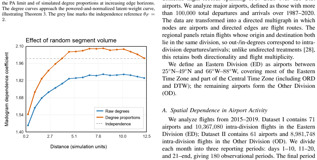
Simulate the model with spatially independent weights but random segment volume: the paper's Remark 2 predicts raw-degree madogram dependence below the independence reference at long distances, while volume-normalized proportions return to independence; a second simulation with constant segment volume should show no long-range raw-degree dependence. Empirically, the decisive check is whether delay or cancellation co-exceedance among airport pairs within roughly 150 km survives conditioning on total system volume and decays toward the baseline beyond about 200 km, as the fitted spatial range of
If this is right
- Distance-decaying dependence in latent node attractiveness survives preferential-attachment aggregation, so hub dominance and spatial co-movement can spring from a single generative mechanism.
- Observed segment volume acts as a distance-independent common mode in raw degrees; normalizing by volume (degree proportions) removes it and exposes the short-range latent spatial component.
- Terminal degree counts are enough to invert both channels — out-weights as powered proportions, in-weights via the strictly concave no-self-loop inverse — so the method transfers to other networks without ordered edge histories.
- Long-run degree proportions cannot identify the attachment exponent; only ordered edge histories (or calibrated dynamic estimates) constrain α, and the data are consistent with a weak exponent near 0.15–0.2.
- In U.S. domestic flights, raw long-distance degree dependence is mostly explained by period volume, and the residual spatial component has an e-folding range of about 74 km (Eastern) and 110 km (Other Division); several European carriers replicate the decomposition.
Where Pith is reading between the lines
- If the decomposition generalizes, raw-degree dependence at long distances in other activity networks (delays, outages, disease counts) may be a segment-volume artifact rather than spatial coupling, so spatial analyses of such counts should first normalize by total activity.
- The fixed-node framework transfers directly to other scheduled systems such as rail or power grids, where the same diagnostics could test for a comparable short spatial range without assuming an edge-by-edge urn.
- The paper's own observation that out- and in-weight estimates nearly coincide suggests a bivariate out-in field is the natural next step; if fitted, the out-in correlation would become a structural parameter instead of a descriptive outcome.
- The ~150 km co-exceedance scale is a model-derived, exploratory prediction; it could be checked directly in independent data by measuring conditional upper-quantile co-exceedance of delay or cancellation events across airport pairs before fitting any model.
Editorial analysis
A structured set of objections, weighed in public.
Referee Report
Summary. The paper proposes a directed preferential-attachment model on a fixed vertex set, with latent node weights driven by temporally persistent Gaussian-process lognormal fields. For 0<α<1, Theorem 1 gives almost-sure limits for out- and in-degree proportions, Theorem 2 for directed edge frequencies, and Theorem 3 for transfer of spatial dependence to the F-madogram. The paper develops terminal-count inversions (Prop. 3), MM estimation with concavity and convergence results (Thms. 4–5), profile likelihood for α, AR(1) pre-whitening, and a spatial quasi-likelihood. Simulations verify transmission of distance-decaying dependence and a common-mode effect of random segment volume. Applications to U.S. domestic flights and European per-carrier networks decompose raw-degree dependence into a distance-independent volume common mode and a short-range spatial component with estimated ranges about 74–110 km and a co-exceedance scale of roughly 150 km.
Significance. The theoretical core is a genuine contribution: fixed-node directed PA with spatial GP weights, explicit limit maps, a strictly concave in-weight inversion, and a rigorous MM framework are nontrivial and clearly proved in the supplement. The paper is also commendably transparent about several limitations: Remark 2 disclaims exactness of the common-mode approximation, Section VII-B calls α a reference rather than an estimate, Supplement S8 labels the profile intervals conditional, and Section VII-E reports mixed replication results. If the within-segment urn model is accepted for the data, the empirical decomposition is informative. However, the empirical interpretation depends heavily on the segment-reset Pólya-urn assumption for airline schedules, which is not supported by institutional knowledge of airline planning; this affects the abstract's central claim of separating network-wide volume variation from a short-range spatial component.
major comments (2)
- [§III-A, Eq. (6); §VII-B, Eq. (35)] The model assumes each observational segment 'starts from zero within-segment degrees' and generates T_ℓ directed events by the weighted PA probability (6). The airline analysis treats 10-day/11-day monthly periods as such segments and applies the large-horizon inversion (35). For scheduled air transport this generative assumption is questionable: route frequencies are planned, capacities are fixed, and route presence persists across periods; the within-period degree process is not a fresh Pólya-urn started at zero. If the generative assumption fails, the estimated log-weights are a fixed monotone transform of observed proportions up to a common shift, and the subsequent AR(1)+spatial fit estimates the covariance of that transform rather than a structural latent-field parameter. The text labels the co-exceedance analysis 'exploratory' and α a 'reference', but the abstract's claim of sepa
- [§VII-B, Table II; §S8] The reported 95% profile intervals for ξ, e.g. [69.8,77.6] km and [103.6,116.4] km, are conditional on the estimated weights, AR parameters, and the fixed α=0.2; Supplement S8 states they 'do not include uncertainty from weight construction or AR fitting'. Since the estimated range is the headline empirical quantity and feeds the 150 km co-exceedance scale in Section VII-D, the absence of unconditional uncertainty makes the empirical support weaker than the point estimates suggest. Please either implement the full bootstrap described in Section V-E, repeating weight construction, AR fitting, and spatial fitting in every replicate, or explicitly state in the abstract and conclusion that the ranges are conditional estimates rather than unconditional empirical findings.
minor comments (5)
- [Algorithm 2, line 10] The pseudocode says 'α∈[α,α]' in the Brent refinement step; this appears to be a typo. It should be a neighborhood of bα or [α_min, α_max].
- [§VII-A] The final period of each month lasts 8–11 days, introducing an exposure-length component in T_ℓ. The text notes this for the volume coefficient of variation, but the raw-degree madogram analysis in Fig. 3 does not appear to adjust for it. Please state explicitly whether the exposure-length component affects the raw-degree profile or is fully captured by the common-mode interpretation.
- [Table II vs. Table S3] Table II reports ξ in units of 100 km, while Table S3 reports spatial ranges in km. The convention is clear from the captions but easy to misread; please unify the units or state both values in each table.
- [References] Reference [34] (Pham, Sheridan, Shimodaira) duplicates reference [14]. Please consolidate or distinguish the two entries.
- [§VII-D] The co-exceedance simulation transforms simulated residual fields using the model map (12), so the resulting 150 km scale is a model-based prediction implied by the fitted exponential covariance rather than an empirical estimate from observed exceedances. The text calls this exploratory, but the wording 'the fitted residual covariance yields an exploratory co-exceedance scale' could be clearer that the scale is not independently estimated from co-exceedance data.
Circularity Check
No significant circularity: the theoretical results are self-contained, and the empirical inversion is a model-based inference rather than a construction-equivalent prediction.
full rationale
The central theoretical results (Theorems 1–5, Propositions 1–3) are proved in the supplement from stochastic-approximation, urn, and convex-optimization arguments; they do not depend on any prior result by the same authors. Equation (35) is the algebraic inverse of the Theorem 1 limit map, so using terminal degree proportions to reconstruct latent weights is standard latent-variable inference, not a prediction that is forced by the fitted values. The raw-degree/common-mode separation is essentially the identity D = T·Q, but the observed-volume reconstruction D* = T*·Q is a semiparametric comparison that could fail if T and Q were strongly associated; it is not a tautology. The 150 km co-exceedance scale is explicitly described as an exploratory summary of the fitted residual covariance model, not as an out-of-sample empirical prediction. Self-citations, such as Wang & Resnick [22], appear only in related-work or technical remarks and are not load-bearing. The paper also acknowledges the weak identifiability of α and the lack of reliable within-day edge order (Section VII-B), which are limitations on interpretation rather than circular steps.
Axiom & Free-Parameter Ledger
free parameters (4)
- PA exponent α =
0.2 (reference; calibrated, not estimated on the same data)
- AR(1) persistence φ (out/in, ED/OD) =
0.934 (ED out/in), 0.917/0.920 (OD out/in)
- Stationary spatial variance γ (out/in) =
ED 0.0274/0.0281; OD 0.0242/0.0249
- Spatial range ξ (out/in) =
ED 73.6/72.9 km; OD 109.8/109.5 km
axioms (5)
- domain assumption Within each observational segment, edge events are generated by the weighted PA probability (6) with within-segment degrees starting at zero.
- domain assumption Latent out/in log-weights follow the stationary GP-lognormal AR(1) model (1)–(5) with exponential covariance; out/in innovations are independent.
- standard math Stochastic-approximation ODE methods (Benaïm, Pemantle) give a.s. convergence of the urn recursions to the unique attracting equilibrium.
- ad hoc to paper α=0.2 is an adequate reference exponent for the airline analysis, and non-identification of α from terminal proportions does not materially affect range estimates.
- domain assumption F-madogram and madogram-coefficient estimates remain valid descriptive dependence diagnostics under temporally dependent segments when a block bootstrap is used.
read the original abstract
Spatially embedded directed networks, such as airline networks, often exhibit simultaneous high activity at nearby nodes. Preferential attachment (PA) explains hub dominance. We extend it to spatial co-movement through a directed PA model whose out- and in-node weights follow temporally persistent Gaussian-process lognormal fields. Under sublinear PA, out-degree proportions converge to explicit normalized powered weights, whereas self-loop exclusion yields a coupled in-degree limit. We derive a strictly concave inverse that recovers the in-weights from terminal degree proportions. For ordered network histories, we develop a minorization-maximization (MM) weight estimator and profile likelihood for the PA exponent; temporal pre-whitening and a spatial quasi-likelihood estimate the latent covariance. Simulations verify transmission of distance-decaying dependence and show how random segment volume creates a distance-independent common mode in raw degrees. An analysis of U.S. domestic flights (2015-2019) separates network-wide volume variation from a short-range spatial component. An observed-volume reconstruction reproduces the raw-degree common mode, and the fitted field yields an exploratory co-exceedance transition scale of roughly 150 km. A per-carrier analysis of European air traffic also reveals the same decomposition.
Figures



Reference graph
Works this paper leans on
-
[1]
Analysis of the effect of extreme weather on the US domestic air network: A delay and cancellation propagation network approach,
A. Bombelli and J. M. Sallan, “Analysis of the effect of extreme weather on the US domestic air network: A delay and cancellation propagation network approach,”J. Transp. Geogr., vol. 107, art. 103541, 2023
2023
-
[2]
The worldwide air transportation network: Anomalous centrality, community structure, and cities’ global roles,
R. Guimer `a, S. Mossa, A. Turtschi, and L. N. Amaral, “The worldwide air transportation network: Anomalous centrality, community structure, and cities’ global roles,”Proc. Natl. Acad. Sci. USA, vol. 102, no. 22, pp. 7794–7799, 2005
2005
-
[3]
The role of the airline transportation network in the prediction and predictability of global epidemics,
V . Colizza, A. Barrat, M. Barth ´elemy, and A. Vespignani, “The role of the airline transportation network in the prediction and predictability of global epidemics,”Proc. Natl. Acad. Sci. USA, vol. 103, no. 7, pp. 2015– 2020, 2006
2015
-
[4]
The hidden geometry of complex, network-driven contagion phenomena,
D. Brockmann and D. Helbing, “The hidden geometry of complex, network-driven contagion phenomena,”Science, vol. 342, no. 6164, pp. 1337–1342, 2013
2013
-
[5]
Emergence of scaling in random net- works,
A.-L. Barab ´asi and R. Albert, “Emergence of scaling in random net- works,”Science, vol. 286, no. 5439, pp. 509–512, 1999
1999
-
[6]
van der Hofstad,Random Graphs and Complex Networks, vol
R. van der Hofstad,Random Graphs and Complex Networks, vol. 1. Cambridge, U.K.: Cambridge Univ. Press, 2016
2016
-
[7]
A geometric preferential attachment model of networks II,
A. D. Flaxman, A. M. Frieze, and J. Vera, “A geometric preferential attachment model of networks II,”Internet Math., vol. 4, no. 1, pp. 87– 111, 2007
2007
-
[8]
Spatial networks,
M. Barth ´elemy, “Spatial networks,”Phys. Rep., vol. 499, no. 1–3, pp. 1– 101, 2011
2011
-
[9]
Geometric inhomogeneous random graphs,
K. Bringmann, R. Keusch, and J. Lengler, “Geometric inhomogeneous random graphs,”Theor. Comput. Sci., vol. 760, pp. 35–54, 2019
2019
-
[10]
Statistics for near independence in multivariate extreme values,
A. W. Ledford and J. A. Tawn, “Statistics for near independence in multivariate extreme values,”Biometrika, vol. 83, no. 1, pp. 169–187, 1996
1996
-
[11]
A dependence measure for multivari- ate and spatial extreme values: Properties and inference,
M. Schlather and J. A. Tawn, “A dependence measure for multivari- ate and spatial extreme values: Properties and inference,”Biometrika, vol. 90, no. 1, pp. 139–156, 2003
2003
-
[12]
Variograms for spatial max-stable random fields,
D. Cooley, P. Naveau, and P. Poncet, “Variograms for spatial max-stable random fields,” inDependence in Probability and Statistics. Springer, 2006, pp. 373–390
2006
-
[13]
Fitting the linear preferential attachment model,
P. Wan, T. Wang, R. A. Davis, and S. I. Resnick, “Fitting the linear preferential attachment model,”Electron. J. Statist., vol. 11, no. 2, pp. 3738–3780, 2017
2017
-
[14]
Joint estimation of prefer- ential attachment and node fitness in growing complex networks,
T. Pham, P. Sheridan, and H. Shimodaira, “Joint estimation of prefer- ential attachment and node fitness in growing complex networks,”Sci. Rep., vol. 6, art. 32558, 2016
2016
-
[15]
On-time performance data,
U.S. Department of Transportation, Bureau of Transportation Statistics, “On-time performance data,” TranStats. [Online]. Available: https:// www.transtats.bts.gov/ONTIME/. Accessed: Jun. 30, 2026
2026
-
[16]
Crowdsourced air traffic data from the OpenSky Network 2019–2020,
M. Strohmeier, X. Olive, J. L ¨ubbe, M. Sch ¨afer, and V . Lenders, “Crowdsourced air traffic data from the OpenSky Network 2019–2020,” Earth Syst. Sci. Data, vol. 13, no. 2, pp. 357–366, 2021
2019
-
[17]
OpenSky Network flight list data,
OpenSky Network, “OpenSky Network flight list data,” Zenodo, 2021. [Online]. Available: https://doi.org/10.5281/zenodo.3931948. Accessed: Jun. 30, 2026
-
[18]
Competition and multiscaling in evolving networks,
G. Bianconi and A.-L. Barab ´asi, “Competition and multiscaling in evolving networks,”Europhys. Lett., vol. 54, no. 4, pp. 436–442, 2001
2001
-
[19]
Scale- free networks from varying vertex intrinsic fitness,
G. Caldarelli, A. Capocci, P. De Los Rios, and M. A. Mu ˜noz, “Scale- free networks from varying vertex intrinsic fitness,”Phys. Rev. Lett., vol. 89, no. 25, art. 258702, 2002
2002
-
[20]
Generalizations of P ´olya’s urn problem,
F. Chung, S. Handjani, and D. Jungreis, “Generalizations of P ´olya’s urn problem,”Ann. Comb., vol. 7, no. 2, pp. 141–153, 2003
2003
-
[21]
Statistical modeling of spatial extremes,
A. C. Davison, S. A. Padoan, and M. Ribatet, “Statistical modeling of spatial extremes,”Statist. Sci., vol. 27, no. 2, pp. 161–186, 2012
2012
-
[22]
Poisson edge growth and preferential attachment networks,
T. Wang and S. I. Resnick, “Poisson edge growth and preferential attachment networks,”Methodol. Comput. Appl. Probab., vol. 25, no. 1, art. 8, 2023
2023
-
[23]
Banerjee, B
S. Banerjee, B. P. Carlin, and A. E. Gelfand,Hierarchical Modeling and Analysis for Spatial Data, 2nd ed. Boca Raton, FL, USA: Chapman & Hall/CRC, 2014
2014
-
[24]
Diestel,Graph Theory, 4th ed
R. Diestel,Graph Theory, 4th ed. Heidelberg, Germany: Springer, 2010
2010
-
[25]
Scale-free networks are rare,
A. D. Broido and A. Clauset, “Scale-free networks are rare,”Nature Commun., vol. 10, art. 1017, 2019
2019
-
[26]
Spatial extremes: Max-stable processes at work,
M. Ribatet, “Spatial extremes: Max-stable processes at work,”J. Soc. Franc ¸aise Statist., vol. 154, no. 2, pp. 156–177, 2013
2013
-
[27]
J. M. Ortega and W. C. Rheinboldt,Iterative Solution of Nonlinear Equations in Several Variables. Philadelphia, PA, USA: SIAM, 2000
2000
-
[28]
Data-driven modeling of systemic air traffic delay propagation: An epidemic model approach,
S. Li, D. Xie, X. Zhang, Z. Zhang, and W. Bai, “Data-driven modeling of systemic air traffic delay propagation: An epidemic model approach,” J. Adv. Transp., vol. 2020, art. 8816615, 2020
2020
-
[29]
Dynamics of stochastic approximation algorithms,
M. Bena ¨ım, “Dynamics of stochastic approximation algorithms,” in S´eminaire de Probabilit ´es XXXIII, Lecture Notes in Mathematics, vol. 1709. Berlin, Germany: Springer, 1999, pp. 1–68
1999
-
[30]
Nonconvergence to unstable points in urn models and stochastic approximations,
R. Pemantle, “Nonconvergence to unstable points in urn models and stochastic approximations,”Ann. Probab., vol. 18, no. 2, pp. 698–712, 1990
1990
-
[31]
Boyd and L
S. Boyd and L. Vandenberghe,Convex Optimization. Cambridge, U.K.: Cambridge Univ. Press, 2004
2004
-
[32]
A new data structure for cumulative frequency tables,
P. M. Fenwick, “A new data structure for cumulative frequency tables,” Softw. Pract. Exper., vol. 24, no. 3, pp. 327–336, 1994. IEEE TRANSACTIONS ON NETWORK SCIENCE AND ENGINEERING, VOL. XX, NO. X, MONTH YYYY 14
1994
-
[33]
Measuring preferential attach- ment in evolving networks,
H. Jeong, Z. N ´eda, and A.-L. Barab ´asi, “Measuring preferential attach- ment in evolving networks,”Europhys. Lett., vol. 61, no. 4, pp. 567–572, 2003
2003
-
[34]
Joint estimation of prefer- ential attachment and node fitness in growing complex networks,
T. Pham, P. Sheridan, and H. Shimodaira, “Joint estimation of prefer- ential attachment and node fitness in growing complex networks,”Sci. Rep., vol. 6, art. 32558, 2016. IEEE TRANSACTIONS ON NETWORK SCIENCE AND ENGINEERING, VOL. XX, NO. X, MONTH YYYY 15 Supplementary Material Equation, Proposition, Theorem, and Algorithm numbers without the “S” prefix re...
arXiv 2016
discussion (0)
Sign in with ORCID, Apple, or X to comment. Anyone can read and Pith papers without signing in.